Compare inferred L in SuSiE when using different covariance matrices
Last updated: 2025-08-28
Checks: 7 0
Knit directory: Improved_LD_SuSiE/
This reproducible R Markdown analysis was created with workflowr (version 1.7.1). The Checks tab describes the reproducibility checks that were applied when the results were created. The Past versions tab lists the development history.
Great! Since the R Markdown file has been committed to the Git repository, you know the exact version of the code that produced these results.
Great job! The global environment was empty. Objects defined in the global environment can affect the analysis in your R Markdown file in unknown ways. For reproduciblity it’s best to always run the code in an empty environment.
The command set.seed(20250821) was run prior to running
the code in the R Markdown file. Setting a seed ensures that any results
that rely on randomness, e.g. subsampling or permutations, are
reproducible.
Great job! Recording the operating system, R version, and package versions is critical for reproducibility.
Nice! There were no cached chunks for this analysis, so you can be confident that you successfully produced the results during this run.
Great job! Using relative paths to the files within your workflowr project makes it easier to run your code on other machines.
Great! You are using Git for version control. Tracking code development and connecting the code version to the results is critical for reproducibility.
The results in this page were generated with repository version 35b71f6. See the Past versions tab to see a history of the changes made to the R Markdown and HTML files.
Note that you need to be careful to ensure that all relevant files for
the analysis have been committed to Git prior to generating the results
(you can use wflow_publish or
wflow_git_commit). workflowr only checks the R Markdown
file, but you know if there are other scripts or data files that it
depends on. Below is the status of the Git repository when the results
were generated:
Ignored files:
    Ignored:    .DS_Store
Note that any generated files, e.g. HTML, png, CSS, etc., are not included in this status report because it is ok for generated content to have uncommitted changes.
These are the previous versions of the repository in which changes were
made to the R Markdown (analysis/Compare_infer_L.Rmd) and
HTML (docs/Compare_infer_L.html) files. If you’ve
configured a remote Git repository (see ?wflow_git_remote),
click on the hyperlinks in the table below to view the files as they
were in that past version.
| File | Version | Author | Date | Message |
|---|---|---|---|---|
| Rmd | dc5a991 | Dat Do | 2025-08-28 | Infer L analysis |
| html | dc5a991 | Dat Do | 2025-08-28 | Infer L analysis |
| Rmd | 18e5ae1 | Dat Do | 2025-08-27 | add infer L file |
In this experiment, we compare the SuSiE model with true \(L_0 = 4\) and fitted \(L\) from 1 to 10. SuSiE has a notable feature that when fitting with \(L > 4\), the PIP for all CSs after 4 will be diffused because all of the causual SNPs have been picked. Therefore we do not select CSs with low purity, where purity is defined by the minimum pairwise correlation of SNPs in a CS. The inferred \(L\) is defined by the number of CSs that have purity excess a chosen threshold (default = 0.5).
library(susieR)
gtex <- readRDS("data/Thyroid_ENSG00000132855.rds")

num_reps = 200

all_L_infer = array(0, dim=c(5, num_reps, 10))

maf = apply(gtex, 2, function(x) sum(x)/2/length(x))
X0 = gtex[, maf > 0.01]
# dim(X0)
X = na.omit(X0)
# dim(X)
snp_total = ncol(X0)


for (seed in 1:num_reps){
  for (L in 1:10){
    # print(seed)
    set.seed(seed)
    n = nrow(X0)
    # Remove SNPs with MAF < 0.01
    p = 200
    min_cor = 0.5
    # Start from a random point on the genome
    indx_start = sample(1: (snp_total - p), 1)
    X = X0[, indx_start:(indx_start + p -1)]
    # View(cor(X)[1:10, 1:10])

    ## sub-sample into two
    out_sample = sample(1:n, 100)
    X_out = X[out_sample, ]
    X_in = X[setdiff(1:n, out_sample), ]
    sum(is.na(X_out))

    rm_p = c(which(diag(cov(X_in))==0), which(diag(cov(X_out))==0))
    length(rm_p)
    indx_p = setdiff(1:p, rm_p)
    X_in = X_in[, indx_p]
    X_out = X_out[, indx_p]

    ## Standardize both sample matrices
    X_in <- scale(X_in)
    X_out <- scale(X_out)

    ## out-sample LD matrix
    R_hat = cor(X_out)
    R = cor(X_in)

    ## generate data from in-sample X matrix
    p = ncol(X_in)
    beta <- rep(0,p)
    n = nrow(X_in)
    ## L_true = 4
    truth = c(1, 50, 100, 150)
    beta[truth] <- c(2, 1, -2, 3)
    ## L_true = 1
    # truth = c(100)
    # beta[truth] <- c(2)
    # plot(beta, pch=16, ylab='effect size')
    y <- X_in %*% beta + rnorm(n)
    y = scale(y)

    ## compute summary statistics
    sumstats <- univariate_regression(X_in, y)
    z_scores <- sumstats$betahat / sumstats$sebetahat
    # susie_plot(z_scores, y = "z", b=beta)
    # L = 10 # overfitted


    ## fit the susie-rss model with in-sample R
    fitted_rss1 <- susie_rss(bhat = sumstats$betahat, shat = sumstats$sebetahat, n = n,
                             R = R, var_y = var(y), L = L,
                             estimate_residual_variance = F,
                             min_abs_corr=min_cor)

    summary(fitted_rss1)$cs
    # p1 = susie_plot(fitted_rss1, y="PIP", b=beta)

    ## fit the model with out-sample R
    fitted_rss2 <- susie_rss(bhat = sumstats$betahat, shat = sumstats$sebetahat, n = n,
                             R = R_hat, var_y = var(y), L = L,
                             estimate_residual_variance = F,
                             min_abs_corr=min_cor)
    # will have problem non-positive cov if estimate_residual_variance = TRUE
    summary(fitted_rss2)$cs
    # p2 = susie_plot(fitted_rss2, y="PIP", b=beta) ## miss the true or does not run


    ## adjusted by identity matrix
    lambda = 0.1
    R_hat_lambd = (1-lambda) * R_hat + lambda * diag(p)
    fitted_rss3 <- susie_rss(bhat = sumstats$betahat, shat = sumstats$sebetahat, n = n,
                             R = R_hat_lambd, var_y = var(y), L = L,
                             estimate_residual_variance = F,
                             min_abs_corr=min_cor)
    # will have problem non-positive cov if estimate_residual_variance = TRUE
    # summary(fitted_rss3)$cs
    # susie_plot(fitted_rss3, y="PIP", b=beta)

    ## using truncated SVD
    alph = 1
    XtY = t(X_in) %*% y
    ZZ = XtY %*% t(XtY)
    R_hat_minus = R_hat - alph * ZZ / (n-1)^2
    eigen_R = eigen(R_hat_minus)
    eigen_R$values

    V <- eigen_R$vectors
    D_plus <- diag(pmax(eigen_R$values, 0))

    R_hat_plus <- V %*% D_plus %*% solve(V) + alph * ZZ / (n-1)^2

    fitted_rss4 <- susie_rss(bhat = sumstats$betahat, shat = sumstats$sebetahat, n = n,
                             R = R_hat_plus, var_y = var(y), L = L,
                             estimate_residual_variance = F,
                             min_abs_corr=min_cor)
    # summary(fitted_rss4)$cs
    # susie_plot(fitted_rss4, y="PIP", b=beta)

    ## combine strategy
    lambda = 0.1
    R_hat_plus_diag = (1-lambda) * R_hat_plus + lambda * diag(p)
    fitted_rss5 <- susie_rss(bhat = sumstats$betahat, shat = sumstats$sebetahat, n = n,
                             R = R_hat_plus_diag, var_y = var(y), L = L,
                             estimate_residual_variance = F,
                             min_abs_corr=min_cor)
    # summary(fitted_rss5)$cs
    # susie_plot(fitted_rss5, y="PIP", b=beta)

    L_true = length(truth)
    fitted_rss = list(fitted_rss1, fitted_rss2, fitted_rss3, fitted_rss4, fitted_rss5)
    for (v in 1:5){
      ## coverage = proportion of CS that contains a true casual SNP
      if (is.null(summary(fitted_rss[[v]])$cs)) {
        all_L_infer[v, seed, L] = 0
      } else{
        L_infer = nrow(summary(fitted_rss[[v]])$cs)
        all_L_infer[v, seed, L] = L_infer
      }
    }
  }
}


library(ggplot2)

list_name = c('In-sample', 'Out-sample', 'Regularized', 'Trunc. SVD')
plots = list()
for (i in 1:4){
  m = (all_L_infer[i, , ])
  colnames(m) <- c(1:10)
  means <- colMeans(m)
  sds   <- apply(m, 2, sd)
  df <- data.frame(
    variable =  factor(colnames(m), levels = colnames(m)),
    mean = means,
    sd = sds
  )

  plots[[i]] = ggplot(df, aes(x = variable, y = mean)) +
    geom_point(size = 3, color = "blue") +
    geom_errorbar(aes(ymin = mean - sd, ymax = mean + sd), width = 0.2) +
    labs(title = list_name[i],
         x = "Methods", y = "Mean ± SD")
}

library(patchwork)
wrap_plots(plots, ncol = 2)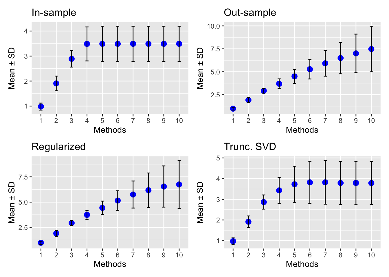
| Version | Author | Date |
|---|---|---|
| dc5a991 | Dat Do | 2025-08-28 |
sessionInfo()R version 4.5.1 (2025-06-13)
Platform: aarch64-apple-darwin20
Running under: macOS Sequoia 15.6.1
Matrix products: default
BLAS: /Library/Frameworks/R.framework/Versions/4.5-arm64/Resources/lib/libRblas.0.dylib
LAPACK: /Library/Frameworks/R.framework/Versions/4.5-arm64/Resources/lib/libRlapack.dylib; LAPACK version 3.12.1
locale:
[1] en_US.UTF-8/en_US.UTF-8/en_US.UTF-8/C/en_US.UTF-8/en_US.UTF-8
time zone: America/Chicago
tzcode source: internal
attached base packages:
[1] stats graphics grDevices utils datasets methods base
other attached packages:
[1] patchwork_1.3.1 ggplot2_3.5.2 susieR_0.14.2 workflowr_1.7.1
loaded via a namespace (and not attached):
[1] sass_0.4.10 generics_0.1.4 stringi_1.8.7 lattice_0.22-7
[5] digest_0.6.37 magrittr_2.0.3 evaluate_1.0.4 grid_4.5.1
[9] RColorBrewer_1.1-3 fastmap_1.2.0 plyr_1.8.9 rprojroot_2.1.0
[13] jsonlite_2.0.0 Matrix_1.7-3 processx_3.8.6 whisker_0.4.1
[17] reshape_0.8.10 ps_1.9.1 mixsqp_0.3-54 promises_1.3.3
[21] httr_1.4.7 scales_1.4.0 jquerylib_0.1.4 cli_3.6.5
[25] rlang_1.1.6 crayon_1.5.3 withr_3.0.2 cachem_1.1.0
[29] yaml_2.3.10 tools_4.5.1 dplyr_1.1.4 httpuv_1.6.16
[33] vctrs_0.6.5 R6_2.6.1 matrixStats_1.5.0 lifecycle_1.0.4
[37] git2r_0.36.2 stringr_1.5.1 fs_1.6.6 irlba_2.3.5.1
[41] pkgconfig_2.0.3 callr_3.7.6 pillar_1.11.0 bslib_0.9.0
[45] later_1.4.2 gtable_0.3.6 glue_1.8.0 Rcpp_1.1.0
[49] xfun_0.52 tibble_3.3.0 tidyselect_1.2.1 rstudioapi_0.17.1
[53] knitr_1.50 farver_2.1.2 htmltools_0.5.8.1 labeling_0.4.3
[57] rmarkdown_2.29 compiler_4.5.1 getPass_0.2-4