Last updated: 2025-08-28

Checks: 7 0

Knit directory: Improved_LD_SuSiE/

This reproducible R Markdown analysis was created with workflowr (version 1.7.1). The Checks tab describes the reproducibility checks that were applied when the results were created. The Past versions tab lists the development history.

R Markdown file: up-to-date

Great! Since the R Markdown file has been committed to the Git repository, you know the exact version of the code that produced these results.

Environment: empty

Great job! The global environment was empty. Objects defined in the global environment can affect the analysis in your R Markdown file in unknown ways. For reproduciblity it’s best to always run the code in an empty environment.

Seed: set.seed(20250821)

The command set.seed(20250821) was run prior to running the code in the R Markdown file. Setting a seed ensures that any results that rely on randomness, e.g. subsampling or permutations, are reproducible.

Session information: recorded

Great job! Recording the operating system, R version, and package versions is critical for reproducibility.

Cache: none

Nice! There were no cached chunks for this analysis, so you can be confident that you successfully produced the results during this run.

File paths: relative

Great job! Using relative paths to the files within your workflowr project makes it easier to run your code on other machines.

Repository version: 35b71f6

Great! You are using Git for version control. Tracking code development and connecting the code version to the results is critical for reproducibility.

The results in this page were generated with repository version 35b71f6. See the Past versions tab to see a history of the changes made to the R Markdown and HTML files.

Note that you need to be careful to ensure that all relevant files for the analysis have been committed to Git prior to generating the results (you can use wflow_publish or wflow_git_commit). workflowr only checks the R Markdown file, but you know if there are other scripts or data files that it depends on. Below is the status of the Git repository when the results were generated:


Ignored files:
    Ignored:    .DS_Store

Untracked files:
    Untracked:  code_push.R

Unstaged changes:
    Modified:   analysis/index.Rmd

Note that any generated files, e.g. HTML, png, CSS, etc., are not included in this status report because it is ok for generated content to have uncommitted changes.

These are the previous versions of the repository in which changes were made to the R Markdown (analysis/Improved_LD_SuSiE_Thyroid_data.Rmd) and HTML (docs/Improved_LD_SuSiE_Thyroid_data.html) files. If you’ve configured a remote Git repository (see ?wflow_git_remote), click on the hyperlinks in the table below to view the files as they were in that past version.

File	Version	Author	Date	Message
Rmd	18e5ae1	Dat Do	2025-08-27	add infer L file
html	521f16a	Ldo3	2025-08-22	Build site.
Rmd	b2d6f17	Ldo3	2025-08-22	wflow_publish("analysis/*")
html	97a384d	Ldo3	2025-08-22	Build site.
Rmd	e01c281	Ldo3	2025-08-22	wflow_publish("analysis/*")
html	21dc38a	Ldo3	2025-08-21	Build site.
Rmd	929c65b	Ldo3	2025-08-21	wflow_publish("analysis/*")
html	7008df9	Ldo3	2025-08-21	Build site.
html	c7b76bb	Ldo3	2025-08-21	Build site.
html	385ca92	Ldo3	2025-08-21	Build site.
Rmd	c2764bb	Ldo3	2025-08-21	Start my new project
html	79c290f	Ldo3	2025-08-21	Build site.
Rmd	eeb4130	Ldo3	2025-08-21	Start my new project
html	1edbb44	Ldo3	2025-08-21	Build site.
Rmd	3ab47e1	Ldo3	2025-08-21	Start my new project

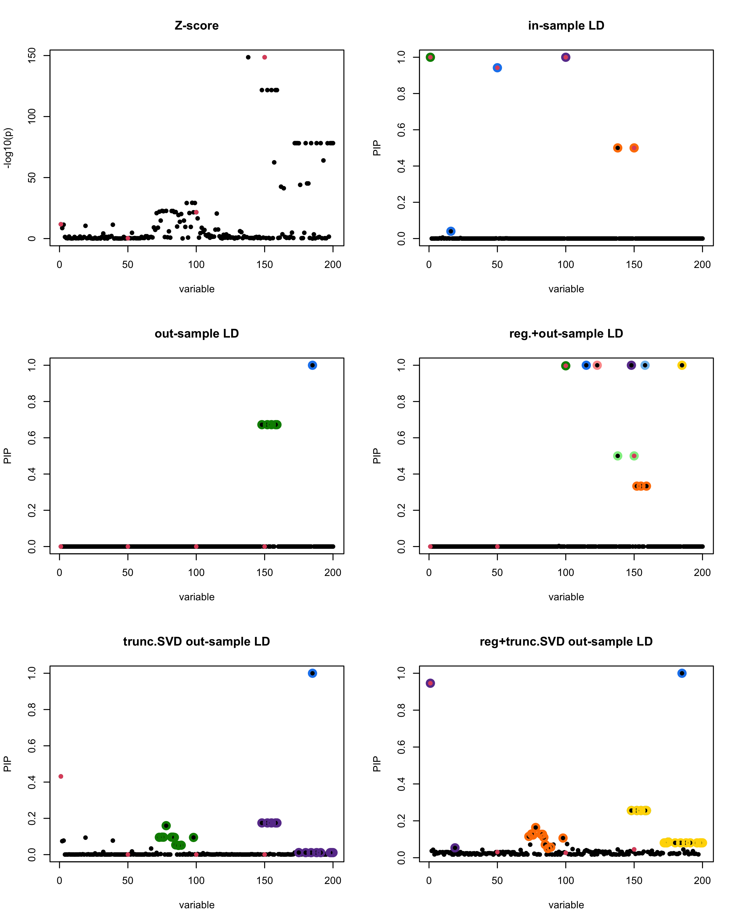
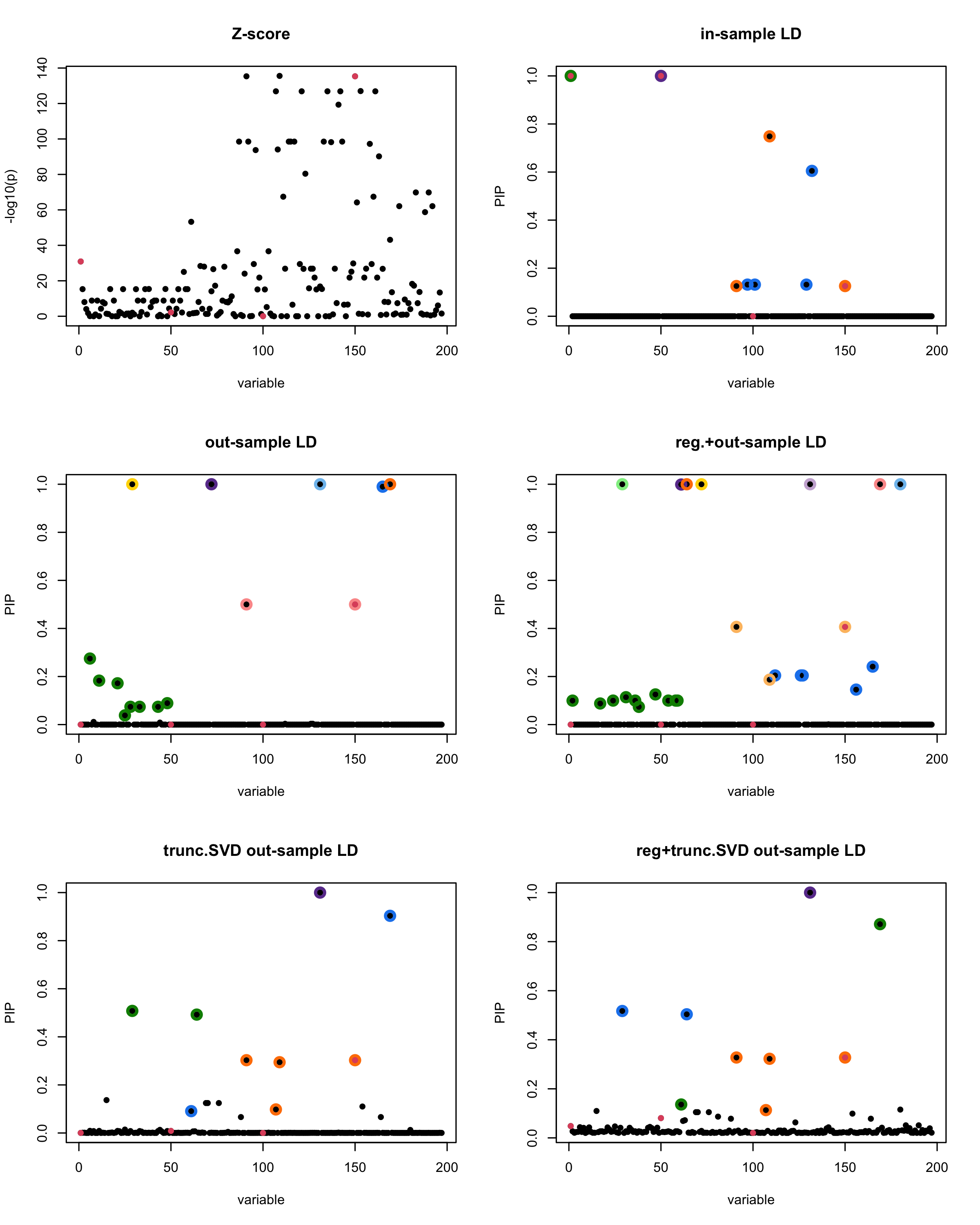
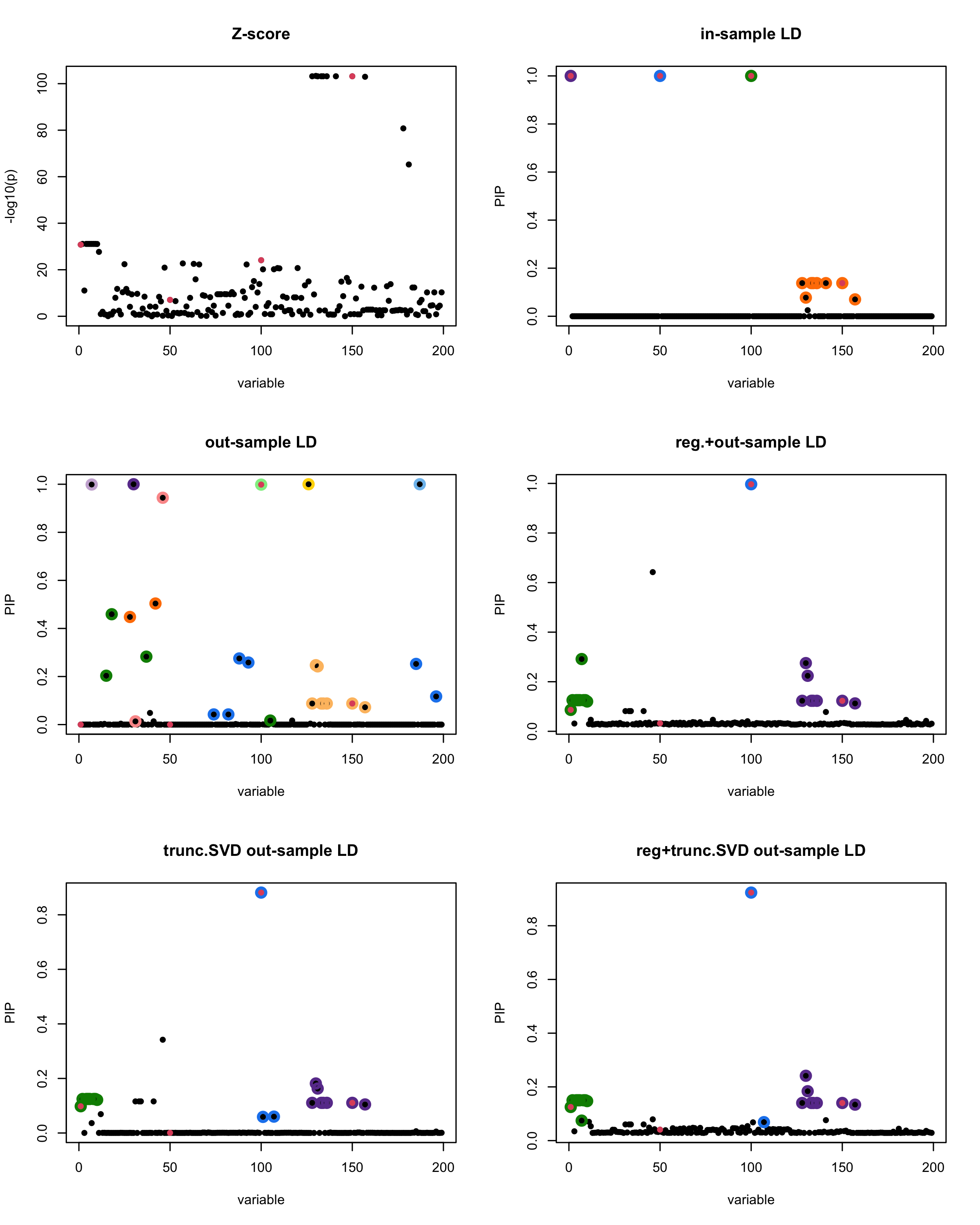
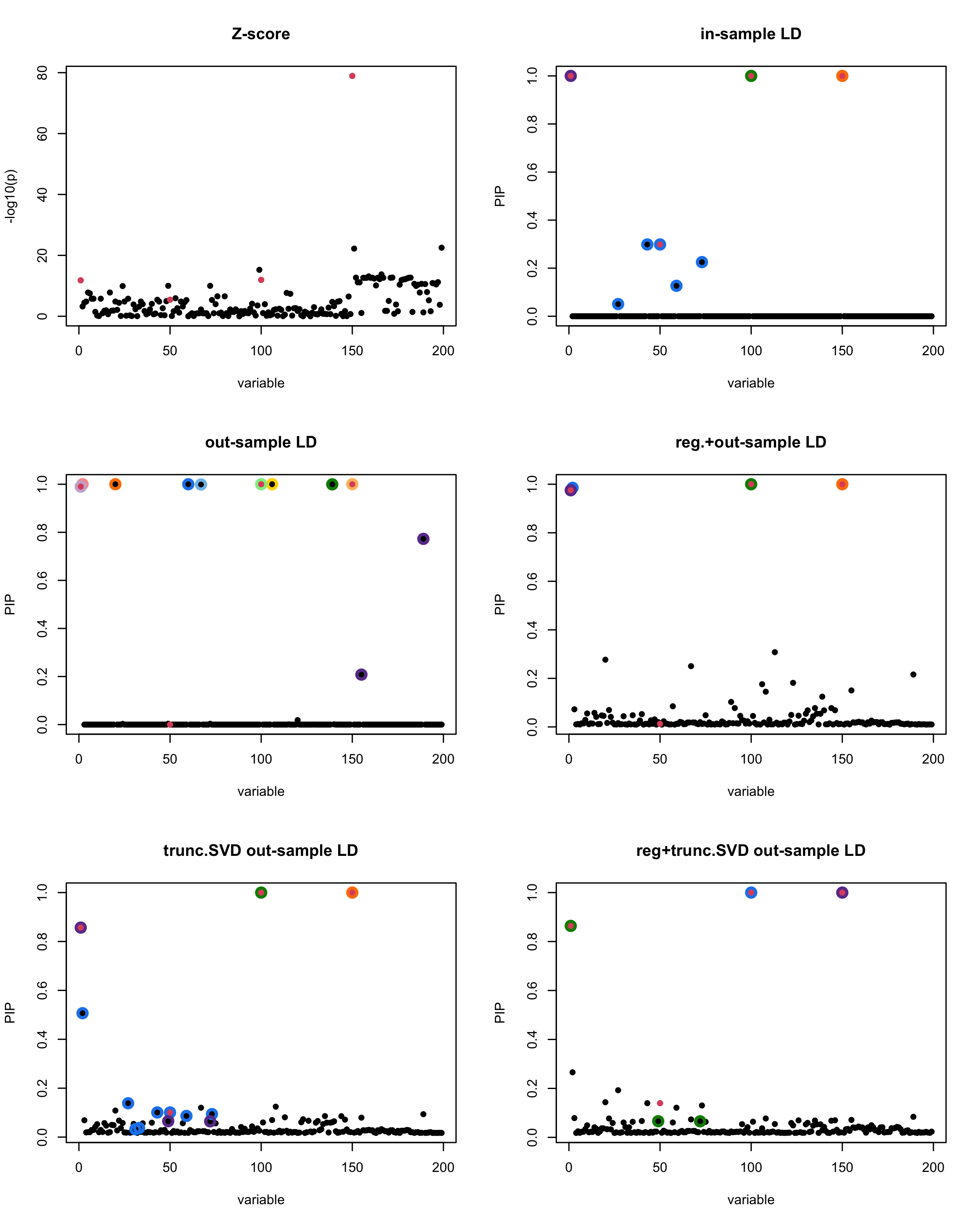
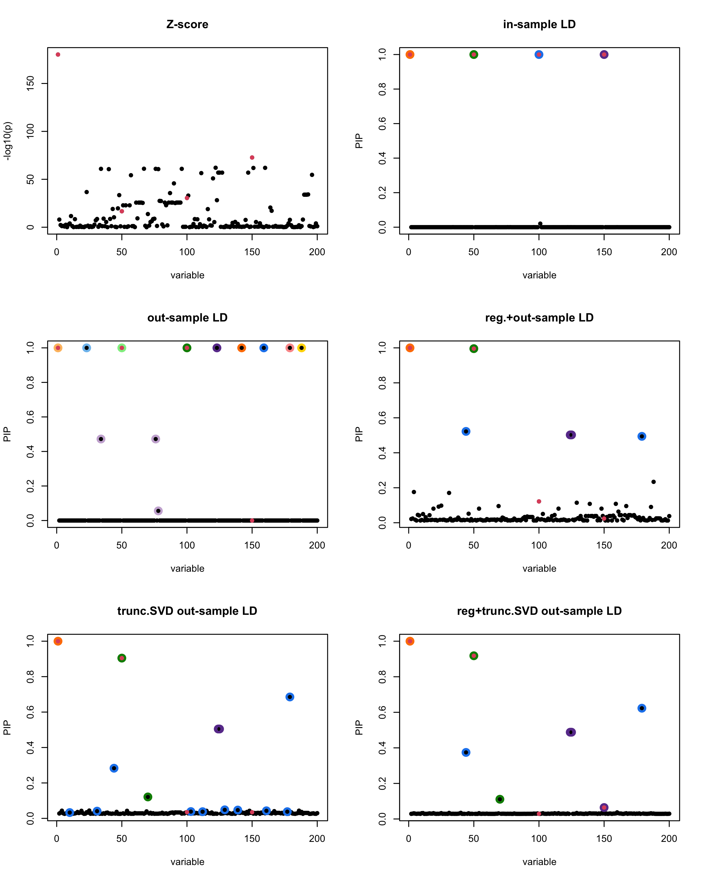
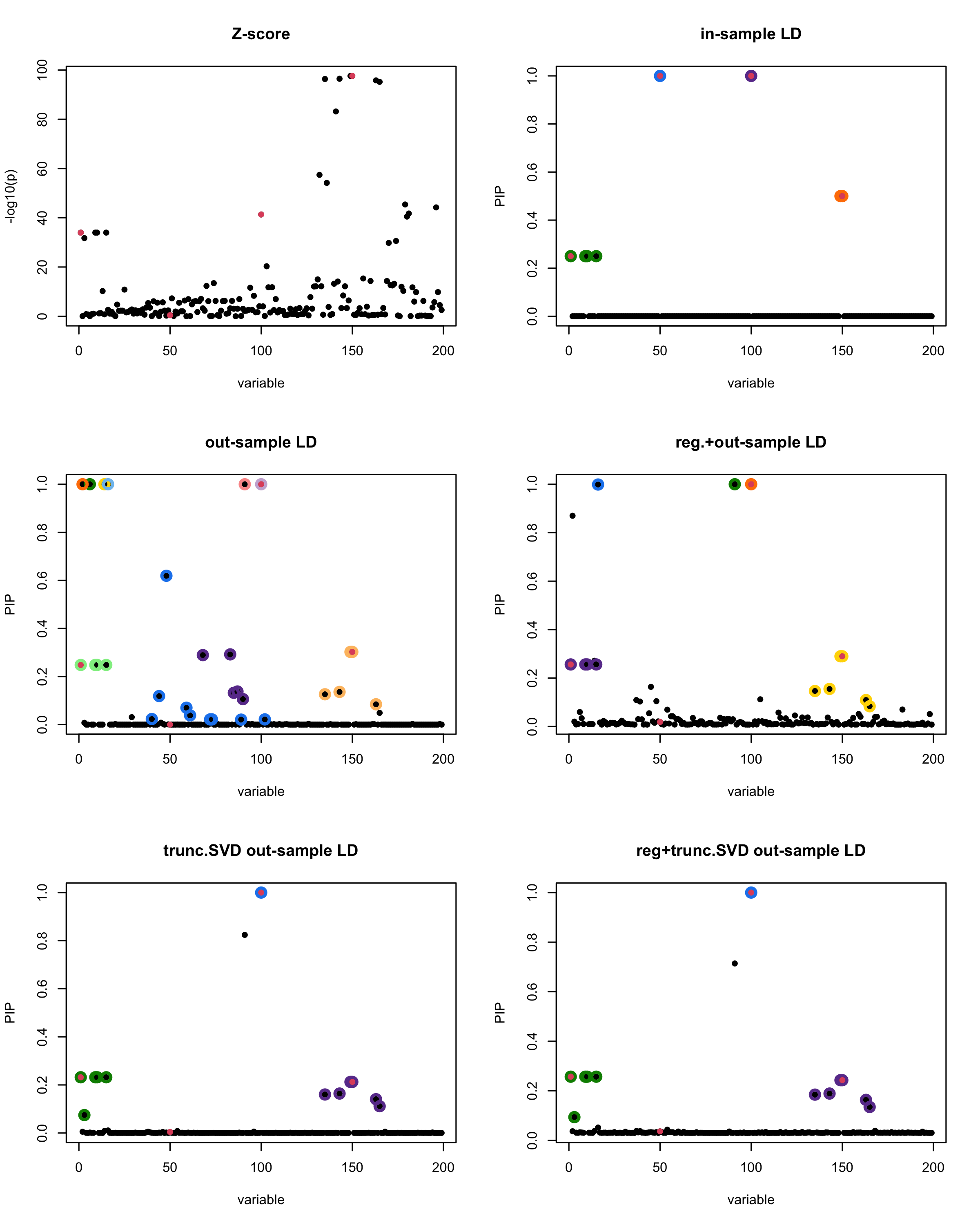
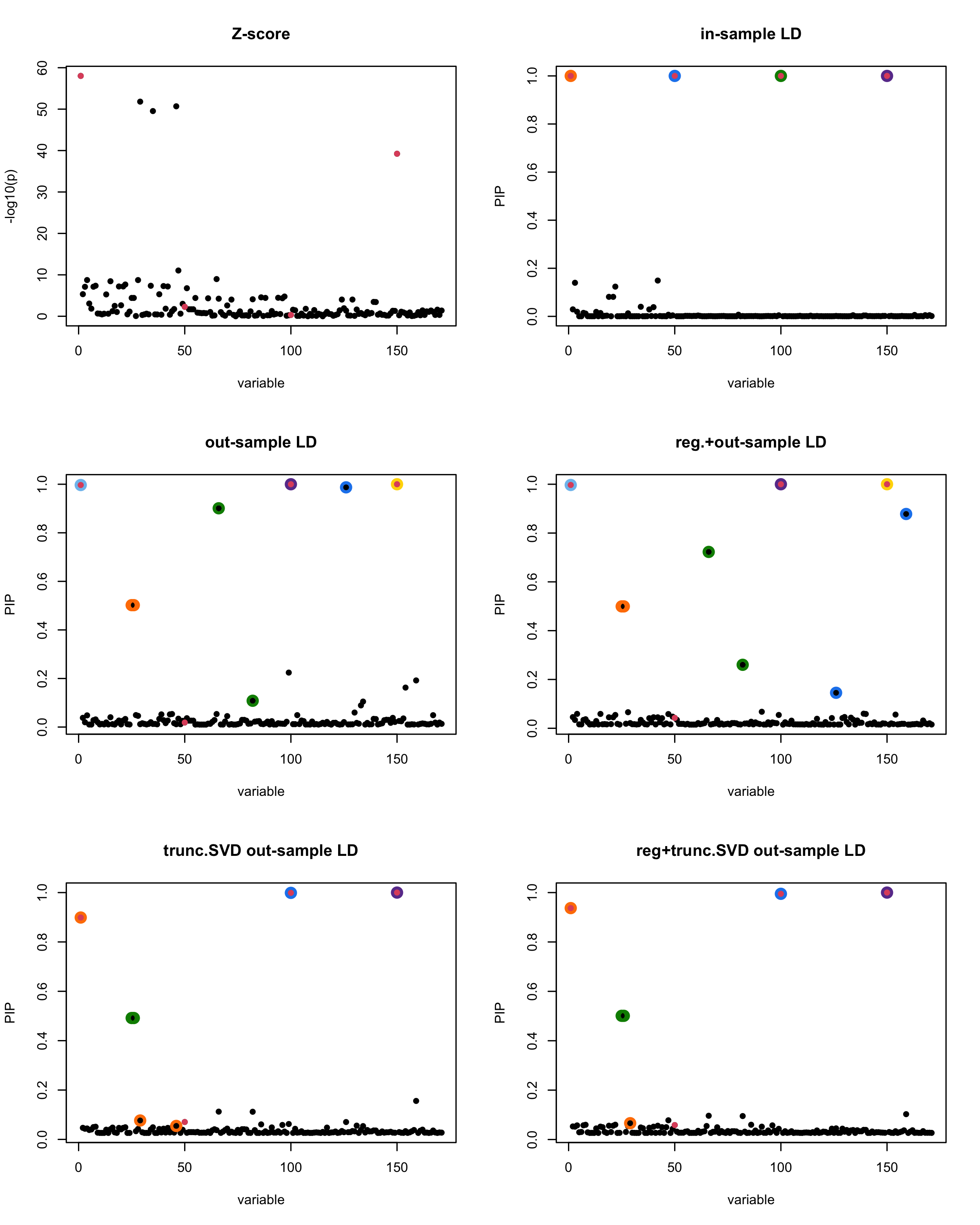
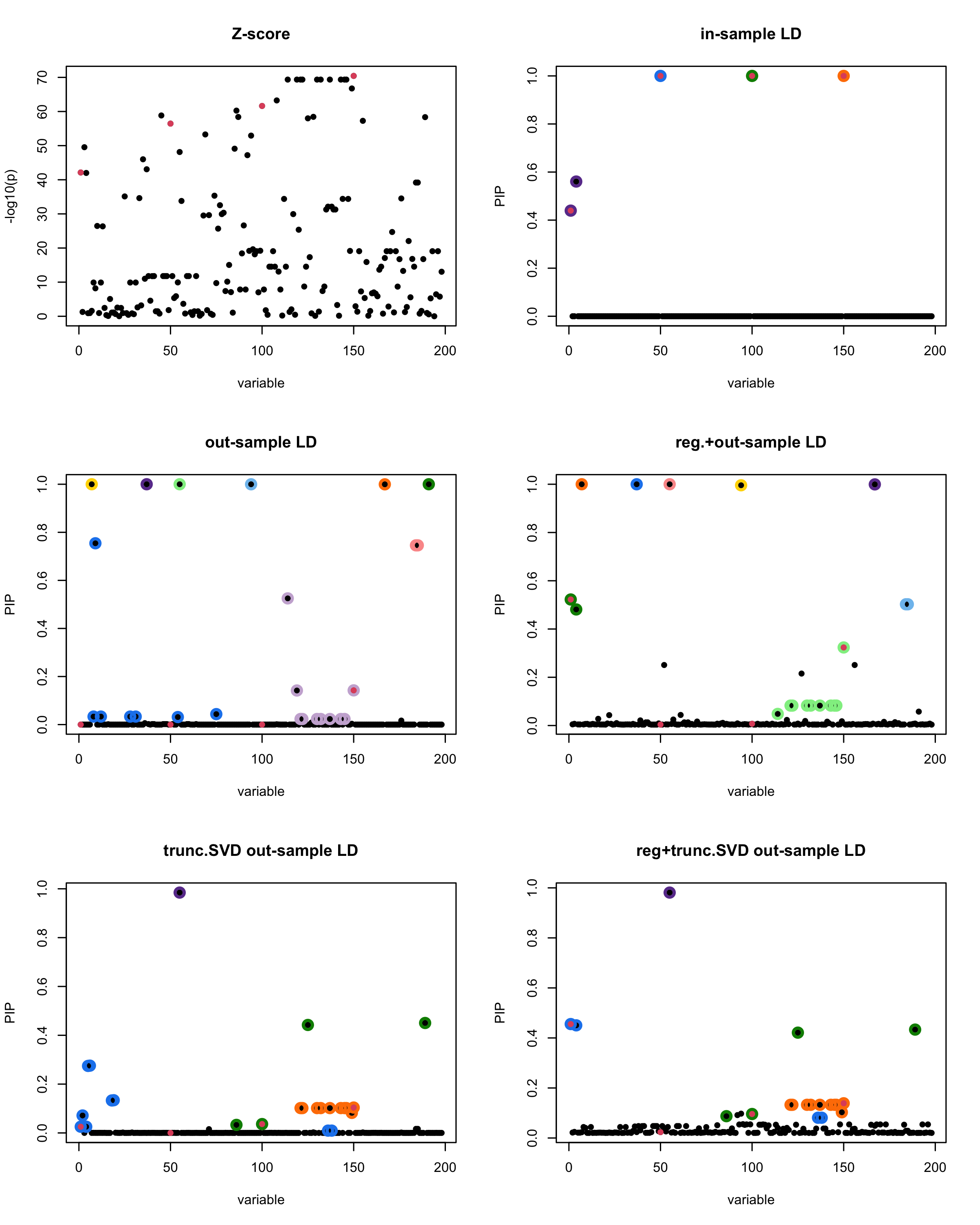
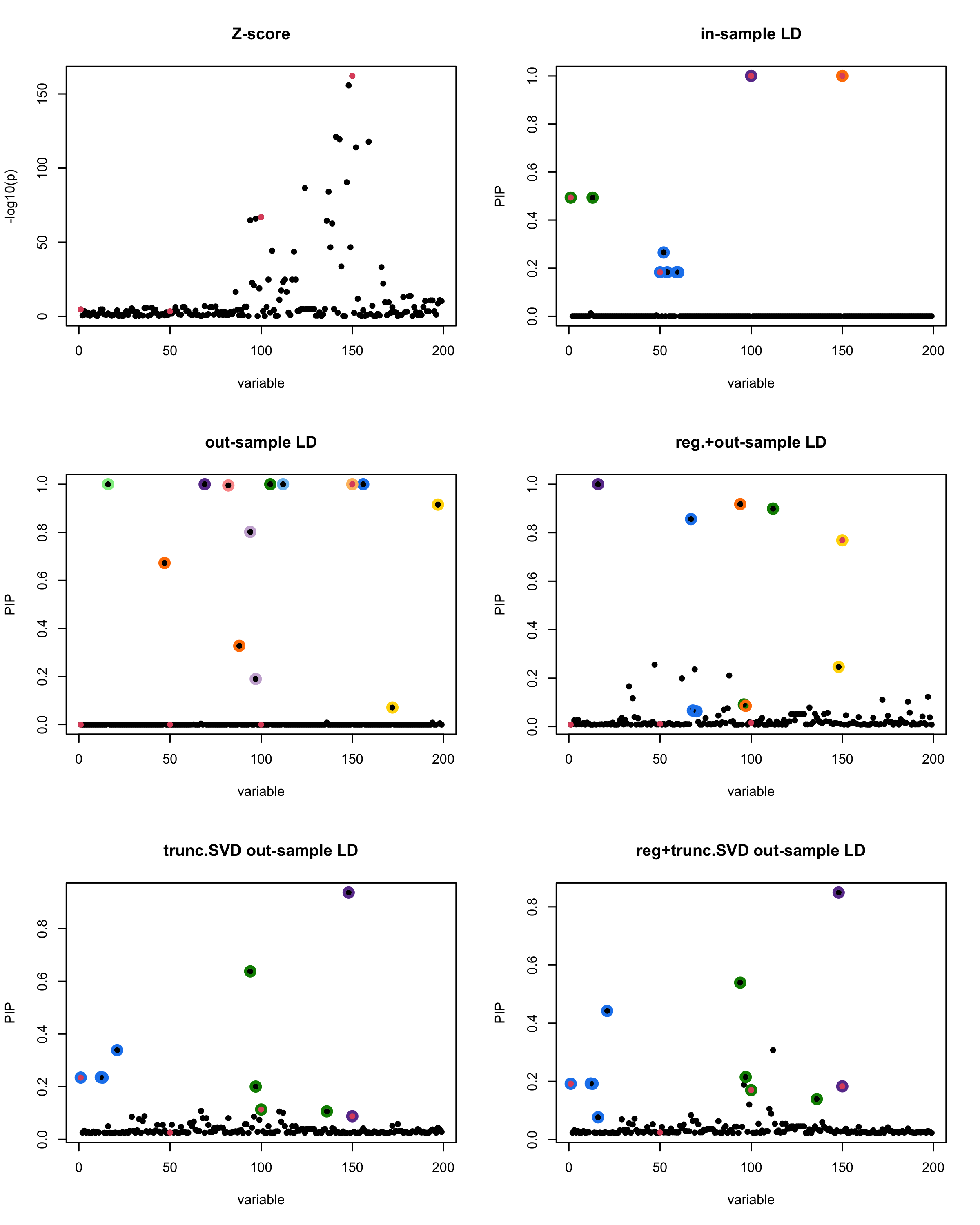
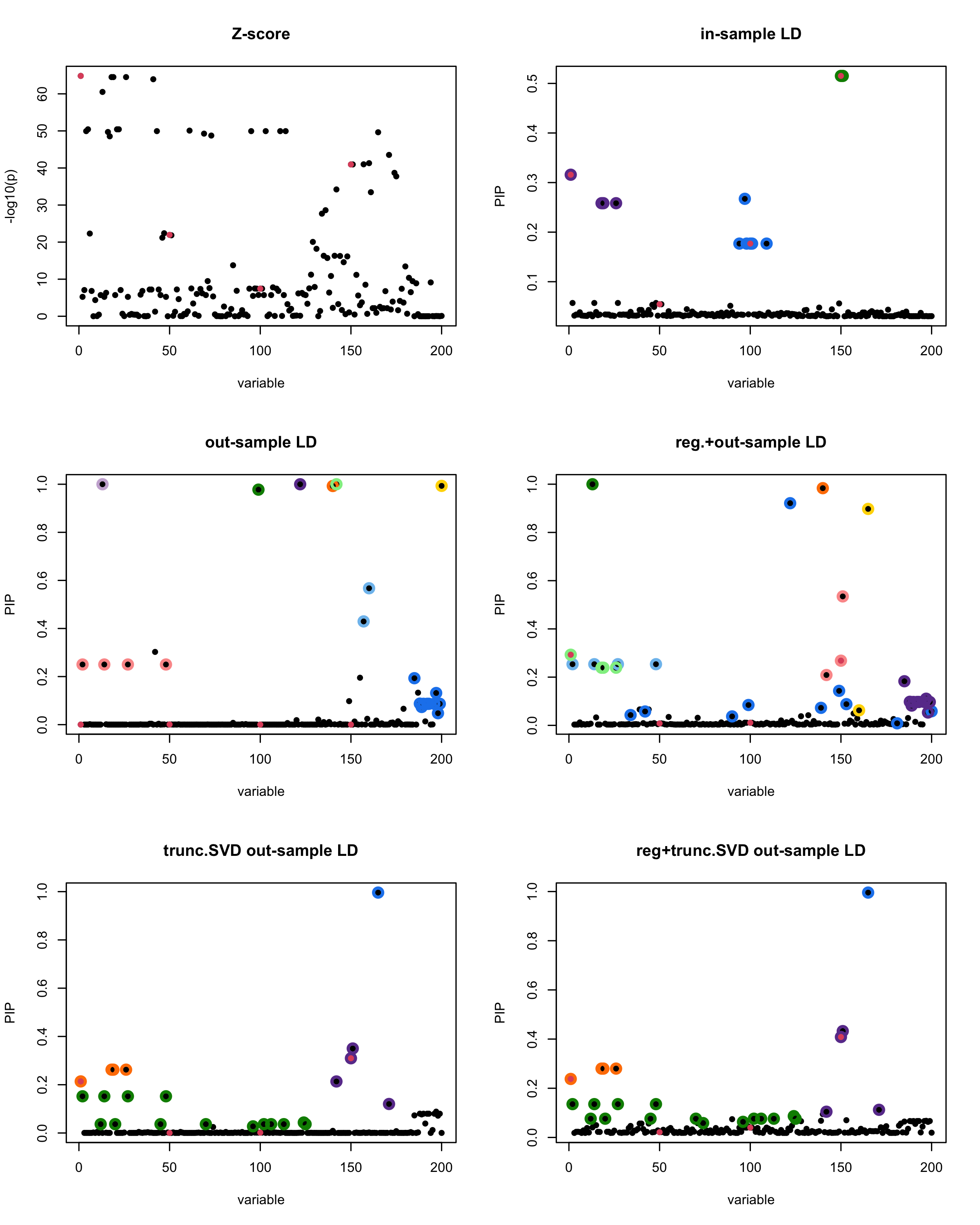
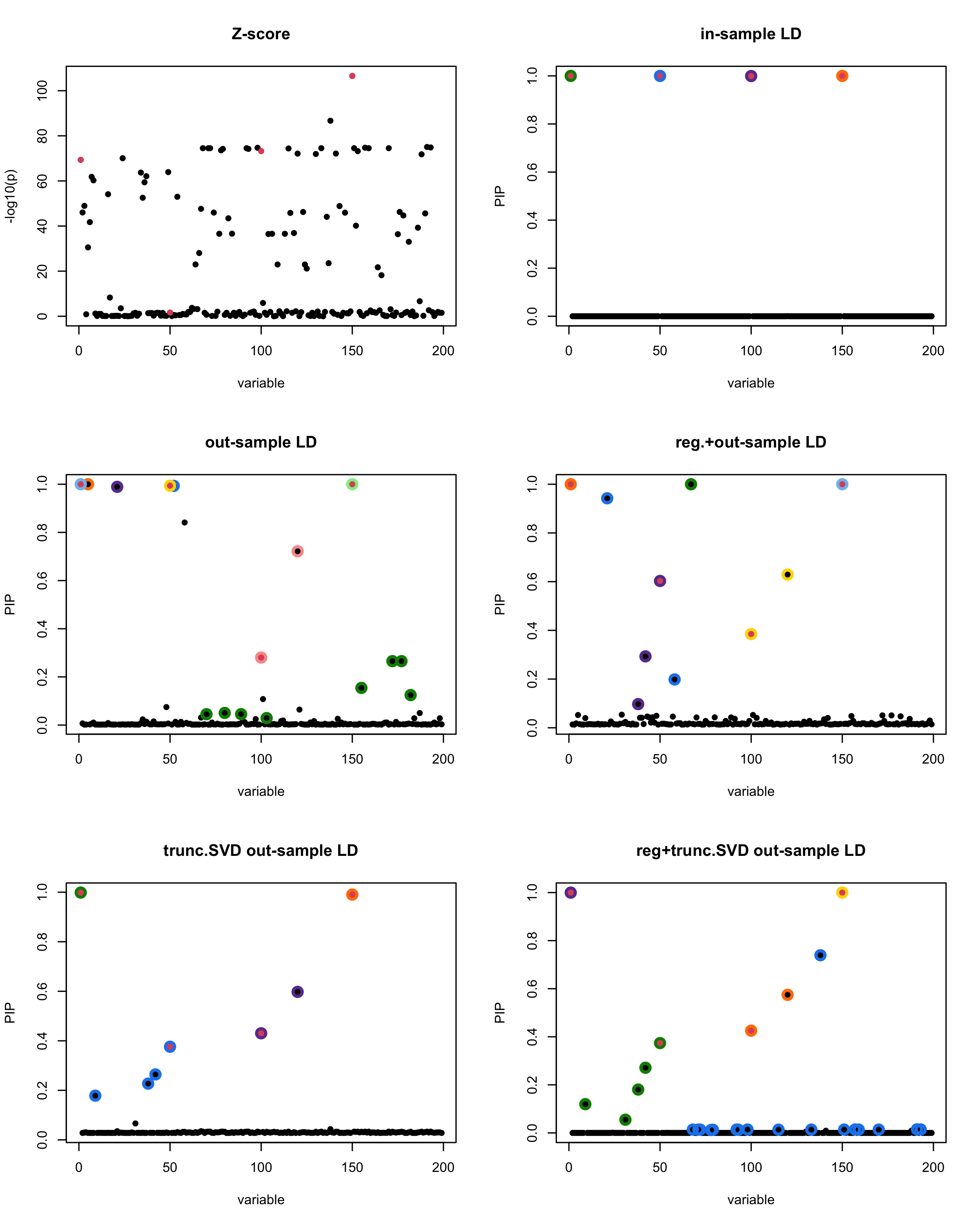
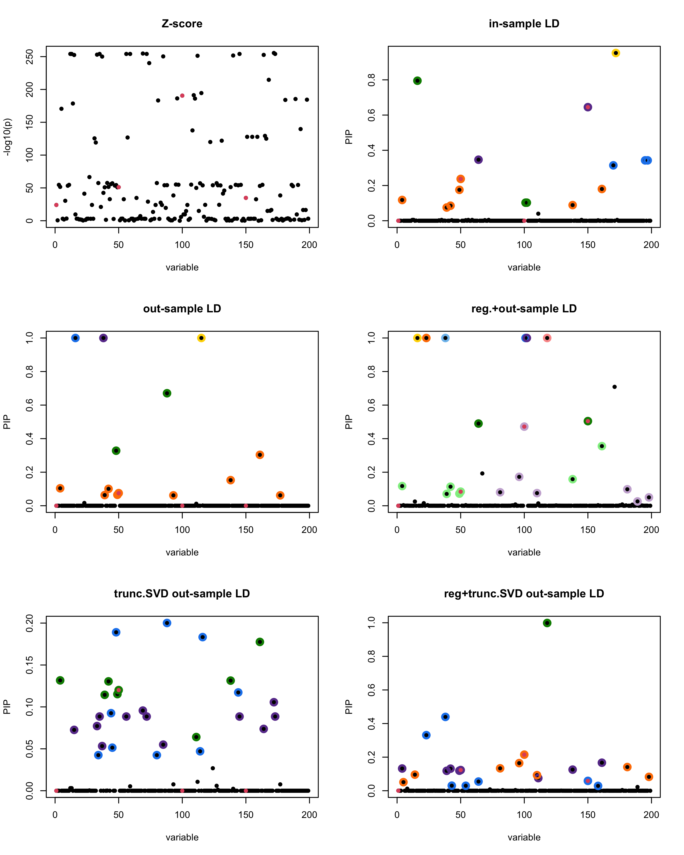
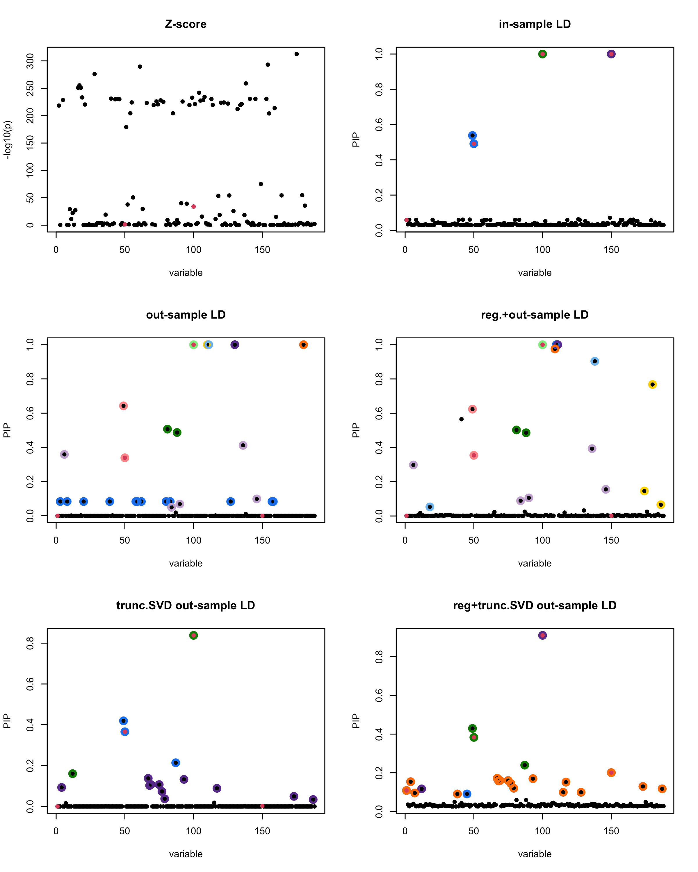
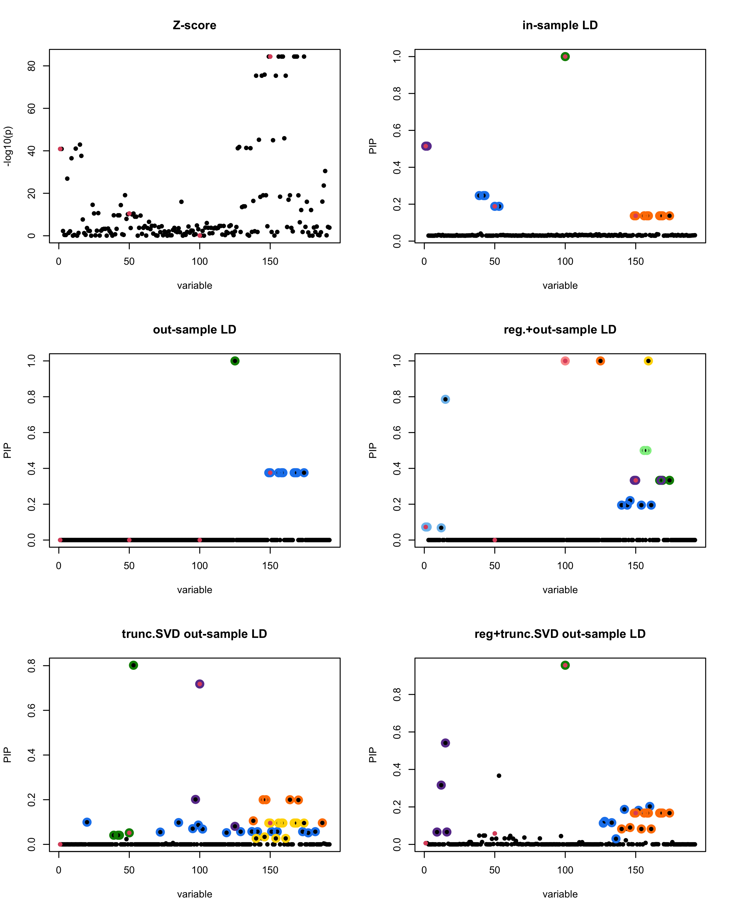
In this experiment, we compare the SuSiE model for summary statistics under different types of the LD matrices. There are 5 types of covariance matrices as we mentioned earlier in the beginning of the page. Let’s recall here once more

In-sample LD matrix: Gold standard
Out-sample LD matrix: LD matrix \(\widehat{R}\) calculated from a out-of-sample data
Regularized: \(\widehat{R}_{\lambda} = (1-\lambda) * \widehat{R} + \lambda * I\) with \(\lambda = 0.1\)
Truncated SVD: \(\tilde{R}\) as presented in the paper
TSVD + Reg.: \(\tilde{R}_{\lambda} = (1-\lambda) * \tilde{R} + \lambda * I\) with \(\lambda = 0.1\)

1. Preprocessing the data and ideas of this experiment

We used the Thyroid data which can be found in the data folder of the source code of this page. The size of the data is \(n \times P\) where \(n = 547\) is the sample size and \(P=7470\) is the total number of SNPs.

library(susieR)
gtex <- readRDS("data/Thyroid_ENSG00000132855.rds")

In the following, we provide the coded-up function for the experiment where the outputs are SuSiE plots with their corresponding LD matrix. In terms of the procedure, we

removed the SNPs with \(MAF < 0.01\),
randomly splitted the Thyroid data into two subsamples called in-sample (\(n_1=474\)) and out-of-sample (\(n_2=100\)) with \(p = 200\). To maintain the correlation between Xs, we subsampled in a way that took consecutive SNPs.
standardized both sample matrices and calculated the out-sample LD matrix.
generated data from the in-sample X matrix where the chosen causal SNPs are in the set \(\{1, 50, 100,150\}\) the corresponding non-zeros \(\beta\)s are \(2,1,-2,3\). Specifically, \[y = X_{\text{in}}\boldsymbol{\beta} + \epsilon, \text{ where } \epsilon \sim \mathcal{N}_{474}(0,\sigma^2I_{474}), \boldsymbol{\beta} = \sum_{l=1}^4\boldsymbol{\beta}_l, \boldsymbol{\beta}_l = \gamma_l\beta_l,\] where \(\gamma_1, \gamma_2, \gamma_3, \gamma_4\) are vectors of all zero but only one value 1 in position \(1, 50, 100, 150\), respectively, and \({\beta_1,\beta_2, \beta_3,\beta_4} = (2,1,-2,3)\). Standardized \(y\).
Fitted univariate regression for \((y, X_{\text{in}})\) and calculated the Z-scores.

Given the known true causal SNPs, we run SuSiE assuming we know nothing about the data but only have the summary statistics.

Let’s see how the different LD matrices affect the detection of causal SNPs.

seed_vary = function(seed)
{
     set.seed(seed)
     print(paste("This is seed number", seed))
     ## good example: seed 3, 4, 8, 10, 11, 12
     ## bad example: seed 5
     # Remove SNPs with MAF < 0.01
     maf = apply(gtex, 2, function(x) sum(x)/2/length(x))
     X0 = gtex[, maf > 0.01]
     dim(X0)
     X = na.omit(X0)
     dim(X)
     snp_total = ncol(X0)
     n = nrow(X0)
     p = 200
     # Start from a random point on the genome
     indx_start = sample(1: (snp_total - p), 1)
     X = X0[, indx_start:(indx_start + p -1)]
     # View(cor(X)[1:10, 1:10])
     
     ## sub-sample into two
     out_sample = sample(1:n, 100)
     X_out = X[out_sample, ]
     X_in = X[setdiff(1:n, out_sample), ]
     sum(is.na(X_out))
     
     rm_p = c(which(diag(cov(X_in))==0), which(diag(cov(X_out))==0))
     length(rm_p)
     indx_p = setdiff(1:p, rm_p)
     X_in = X_in[, indx_p]
     X_out = X_out[, indx_p]
     
     ## Standardize both sample matrices
     X_in <- scale(X_in)
     X_out <- scale(X_out)
     
     ## out-sample LD matrix
     R_hat = cor(X_out)
     R = cor(X_in)
     # View(R_hat[1:10, 1:10])
     # View(R[1:10, 1:10])
     # View(cor(X)[1:10, 1:10])
     
     ## generate data from in-sample X matrix
     p = ncol(X_in)
     beta <- rep(0,p)
     n = nrow(X_in)
     beta[c(1, 50, 100, 150)] <- c(2, 1, -2, 3)
     # plot(beta, pch=16, ylab='effect size')
     y <- X_in %*% beta + rnorm(n)
     y = scale(y)
     
     ## compute summary statistics 
     sumstats <- univariate_regression(X_in, y)
     z_scores <- sumstats$betahat / sumstats$sebetahat
     # susie_plot(z_scores, y = "z", b=beta)
     min_cor = 0.01
     ## fit the susie-rss model with in-sample R
     fitted_rss1 <- susie_rss(bhat = sumstats$betahat, shat = sumstats$sebetahat, n = n, 
                              R = R, var_y = var(y), L = 10,
                              estimate_residual_variance = TRUE,
                              min_abs_corr=min_cor)
     # summary(fitted_rss1)$cs
     # p1 = susie_plot(fitted_rss1, y="PIP", b=beta)
     
     ## fit the model with out-sample R
     fitted_rss2 <- susie_rss(bhat = sumstats$betahat, shat = sumstats$sebetahat, n = n, 
                              R = R_hat, var_y = var(y), L = 10,
                              estimate_residual_variance = FALSE,
                              min_abs_corr=min_cor)
     # will have problem non-positive cov if estimate_residual_variance = TRUE
     # summary(fitted_rss2)$cs
     # p2 = susie_plot(fitted_rss2, y="PIP", b=beta) ## miss the true or does not run
     
     
     ## adjusted by identity matrix
     lambda = 0.1
     R_hat_lambd = (1-lambda) * R_hat + lambda * diag(p)
     fitted_rss3 <- susie_rss(bhat = sumstats$betahat, shat = sumstats$sebetahat, n = n, 
                              R = R_hat_lambd, var_y = var(y), L = 10,
                              estimate_residual_variance = F,
                              min_abs_corr=min_cor)
     # will have problem non-positive cov if estimate_residual_variance = TRUE
     # summary(fitted_rss3)$cs
     # susie_plot(fitted_rss3, y="PIP", b=beta) 
     
     ## using truncated SVD
     alph = 1
     XtY = t(X_in) %*% y
     ZZ = XtY %*% t(XtY) 
     R_hat_minus = R_hat - alph * ZZ / (n-1)^2
     eigen_R = eigen(R_hat_minus)
     eigen_R$values
     
     V <- eigen_R$vectors
     D_plus <- diag(pmax(eigen_R$values, 0))
     
     R_hat_plus <- V %*% D_plus %*% solve(V) + alph * ZZ / (n-1)^2
     
     fitted_rss4 <- susie_rss(bhat = sumstats$betahat, shat = sumstats$sebetahat, n = n, 
                              R = R_hat_plus, var_y = var(y), L = 10,
                              estimate_residual_variance = F,
                              min_abs_corr=min_cor)
     # summary(fitted_rss4)$cs
     # susie_plot(fitted_rss4, y="PIP", b=beta)
     
     ## combine strategy
     lambda = 0.1
     R_hat_plus_diag = (1-lambda) * R_hat_plus + lambda * diag(p)
     fitted_rss5 <- susie_rss(bhat = sumstats$betahat, shat = sumstats$sebetahat, n = n, 
                              R = R_hat_plus_diag, var_y = var(y), L = 10,
                              estimate_residual_variance = F,
                              min_abs_corr=min_cor)
     # summary(fitted_rss5)$cs
     # susie_plot(fitted_rss5, y="PIP", b=beta)
     
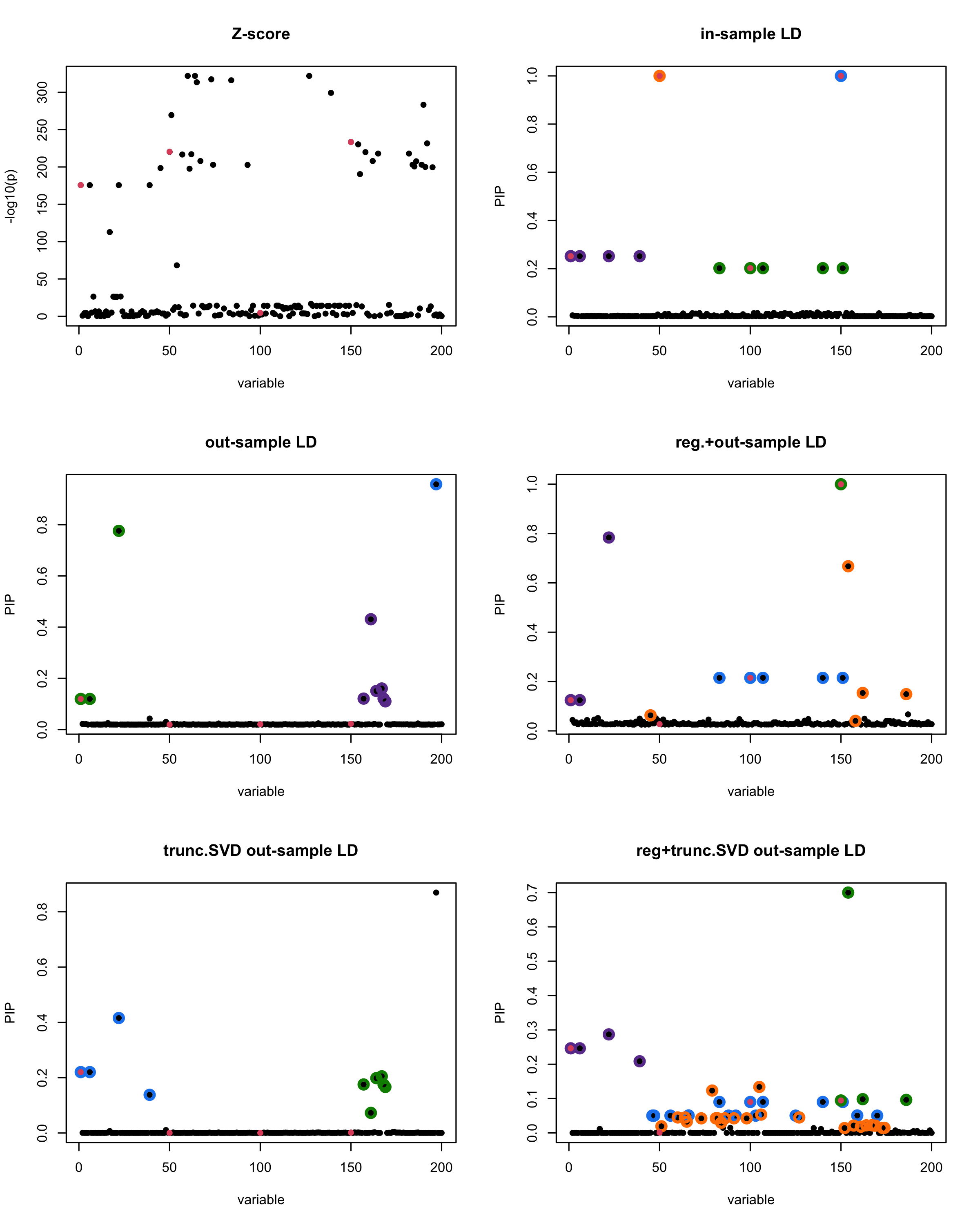
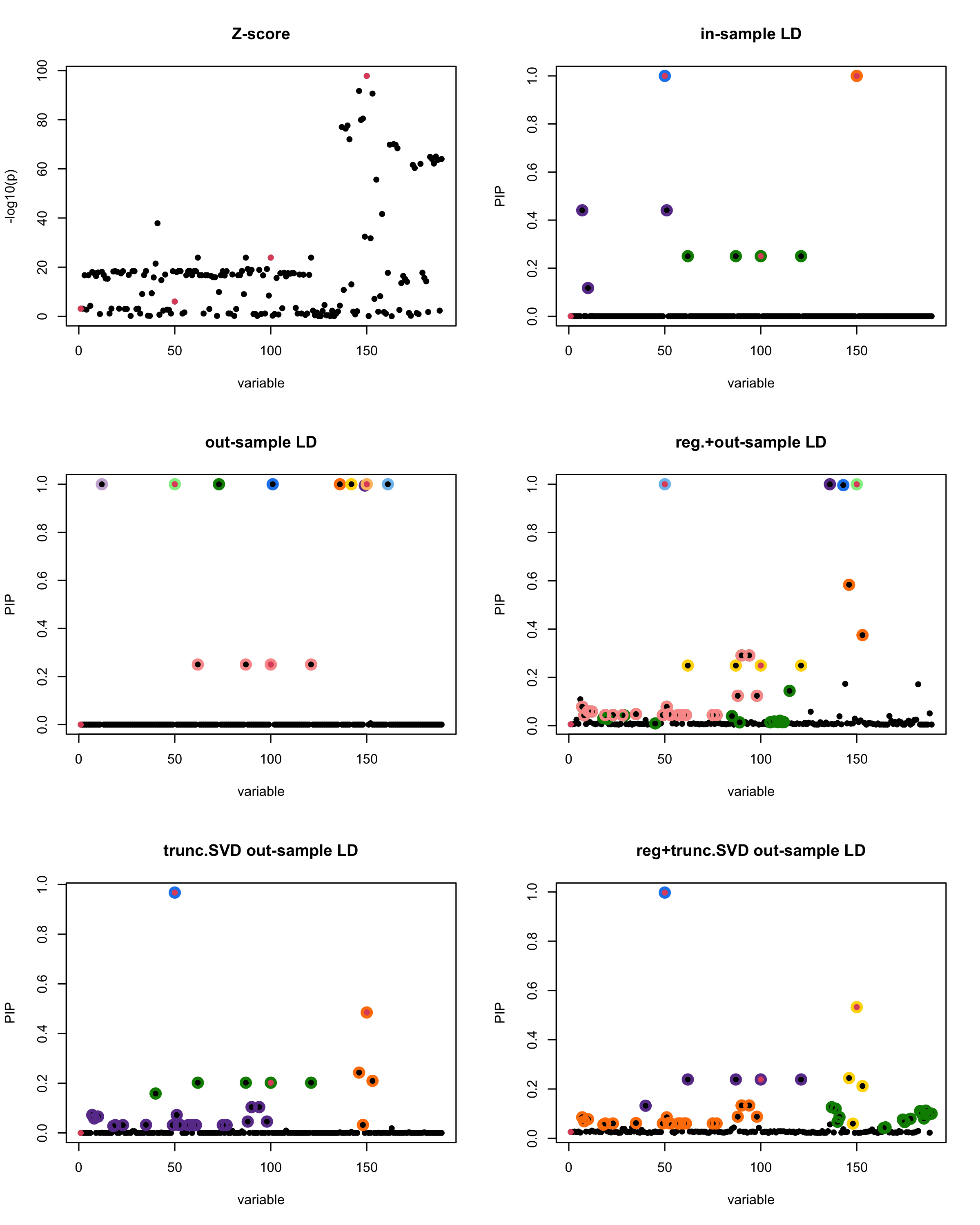
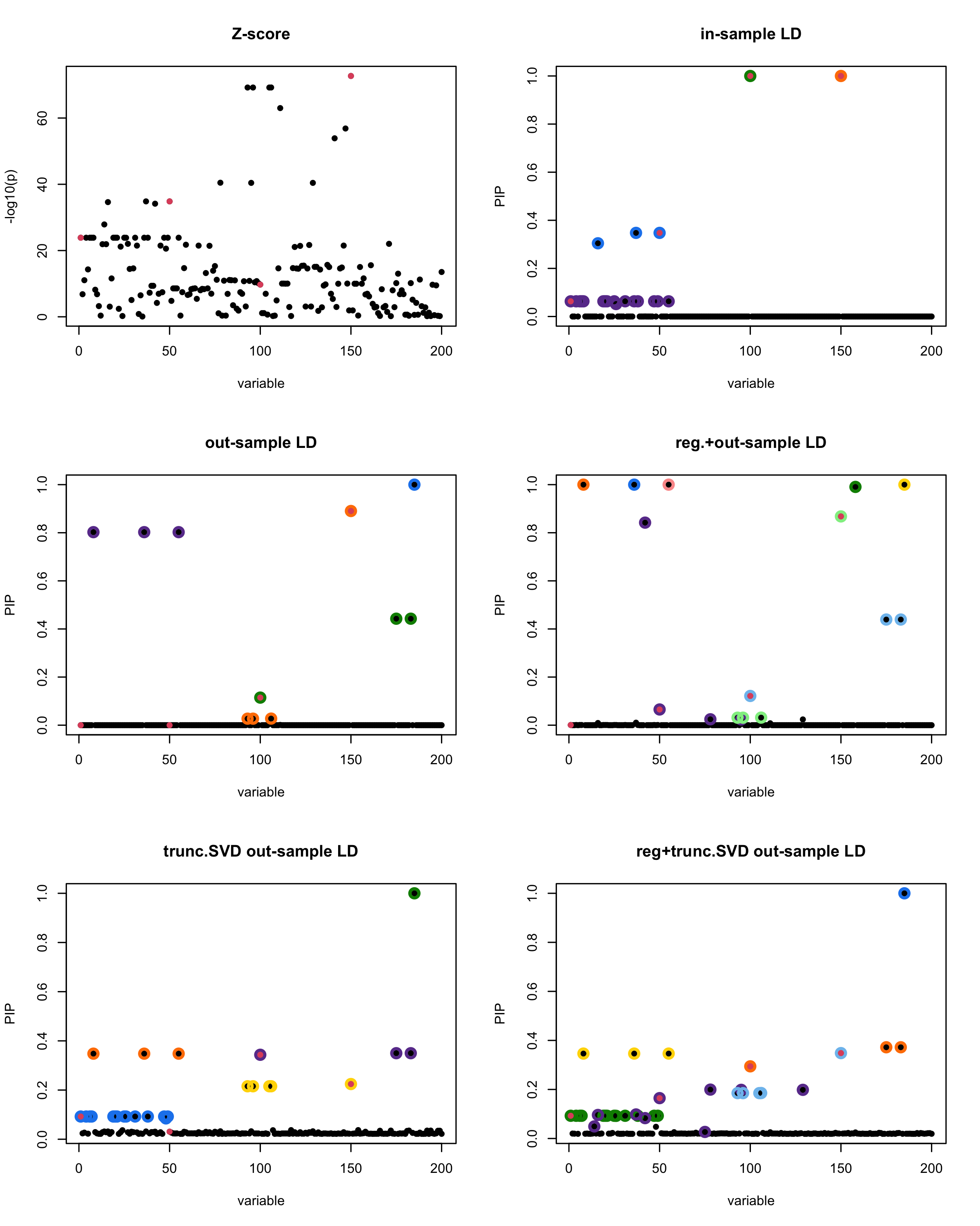
     par(mfrow = c(3, 2))
     susie_plot(z_scores, y = "z", b=beta)
     title('Z-score')
     susie_plot(fitted_rss1, y="PIP", b=beta)
     title('in-sample LD')
     susie_plot(fitted_rss2, y="PIP", b=beta)
     title('out-sample LD')
     susie_plot(fitted_rss3, y="PIP", b=beta)
     title('reg.+out-sample LD')
     susie_plot(fitted_rss4, y="PIP", b=beta)
     title('trunc.SVD out-sample LD')
     susie_plot(fitted_rss5, y="PIP", b=beta)
     title('reg+trunc.SVD out-sample LD')
     print(paste("Minimum eigenvalue is:",min(eigen_R$values,"corresponding to the seed", seed)))
}

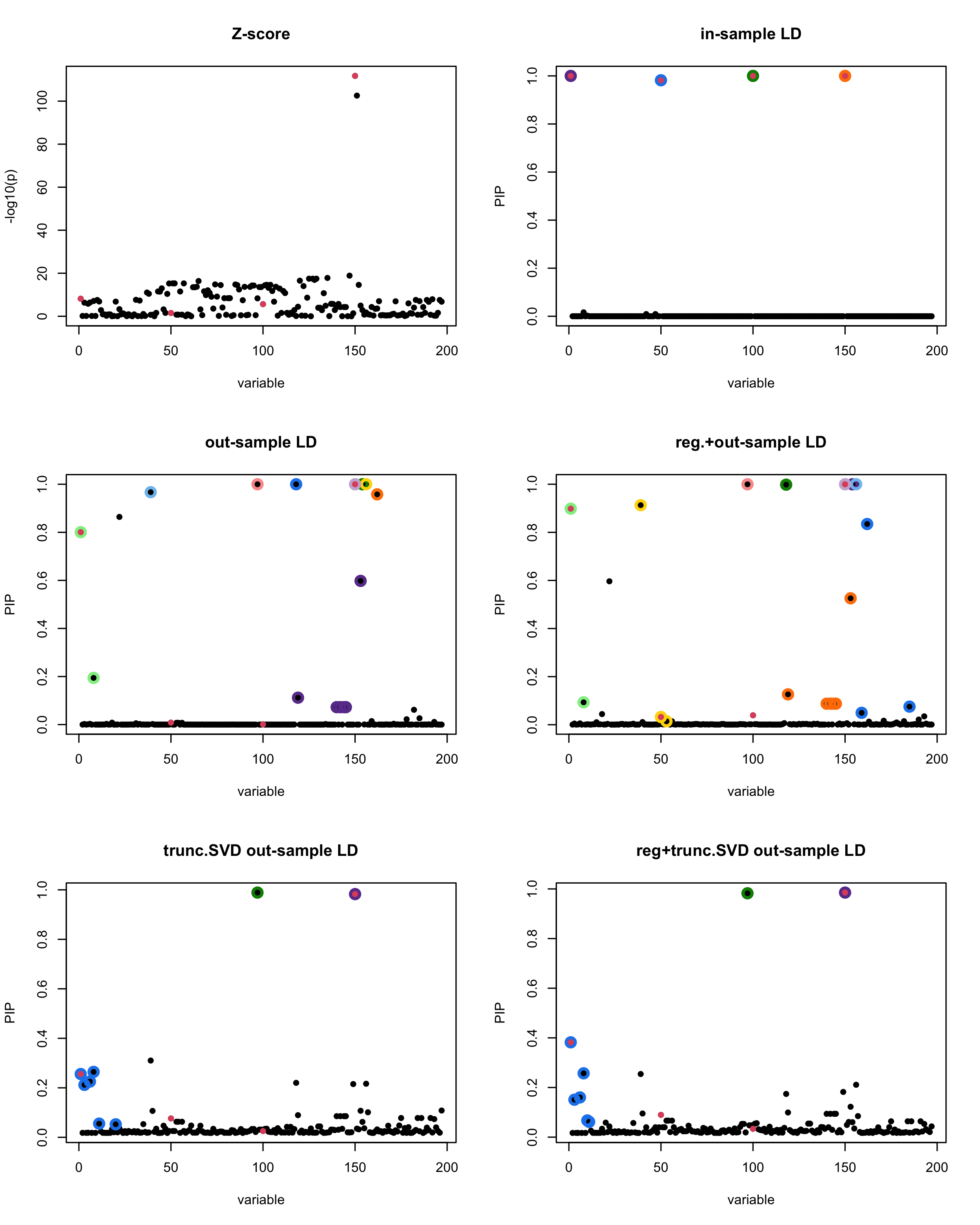
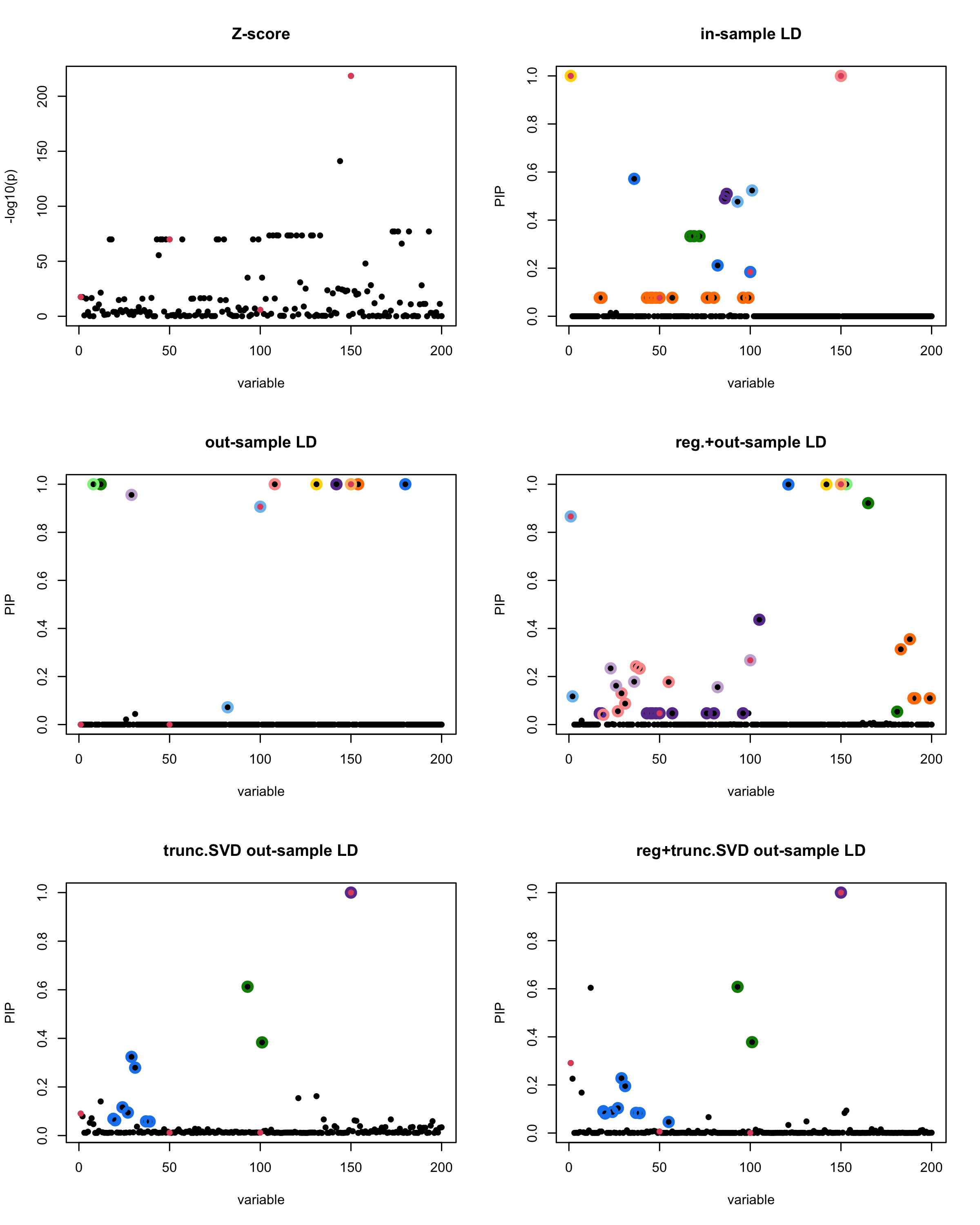
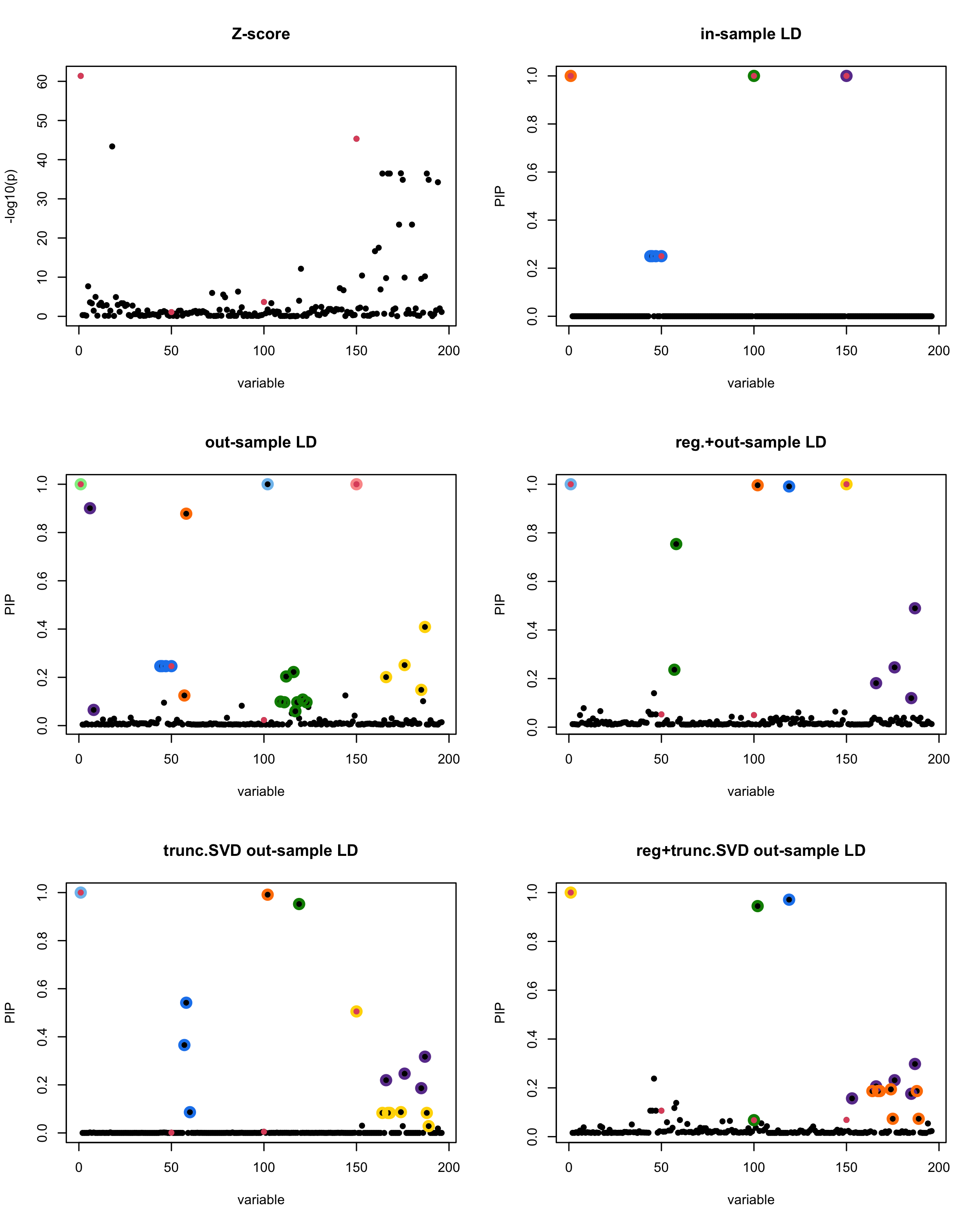
2. Running the experiment with different seed

We vary the random seed to be from \(1-20\).

The following table records cases where the TSVD LD matrix provides a “better,” equal, or worse PIP output compared to the out-sample LD matrix. The “better” here means improving power in detecting the causal SNPs and reducing FDR.

Result	seed 1	seed 2	seed 3	seed 4	seed 5	seed 6	seed 7	seed 8	seed 9	seed 11	seed 12	seed 13	seed 14	seed 15	seed 16	seed 17	seed 18	seed 19	seed 20
better			■	■			▲	▲	▲	■	■	■	▲	▲	▲	⬤	▲
equal		✓				✓
worse	x				x													x	x

Note

■ for cases where the TSVD improved the power and reduce the FDR compare to out-sample LD.
● for cases where the TSVD improved the power but increased the FDR compare to out-sample LD.
▲ for cases where the TSVD maintained the same power but reduced the FDR compare to out-sample LD.

[1] “This is seed number 1”

Version	Author	Date
97a384d	Ldo3	2025-08-22

[1] “Minimum eigenvalue is: -3.711724”

[1] “This is seed number 2”

Version	Author	Date
97a384d	Ldo3	2025-08-22

[1] “Minimum eigenvalue is: -1.989602”

[1] “This is seed number 3”

Version	Author	Date
97a384d	Ldo3	2025-08-22

[1] “Minimum eigenvalue is: -0.9986563”

[1] “This is seed number 4”

Version	Author	Date
97a384d	Ldo3	2025-08-22

[1] “Minimum eigenvalue is: -0.3631381”

[1] “This is seed number 5”

Version	Author	Date
97a384d	Ldo3	2025-08-22

[1] “Minimum eigenvalue is: -0.7655705”

[1] “This is seed number 6”

Version	Author	Date
97a384d	Ldo3	2025-08-22

[1] “Minimum eigenvalue is: -2.874186”

[1] “This is seed number 7”

Version	Author	Date
97a384d	Ldo3	2025-08-22

[1] “Minimum eigenvalue is: -1.981569”

[1] “This is seed number 8”

Version	Author	Date
97a384d	Ldo3	2025-08-22

[1] “Minimum eigenvalue is: -1.601618”

[1] “This is seed number 9”

Version	Author	Date
97a384d	Ldo3	2025-08-22

[1] “Minimum eigenvalue is: -1.278852”

[1] “This is seed number 10”

Version	Author	Date
97a384d	Ldo3	2025-08-22

[1] “Minimum eigenvalue is: -0.4129873”

[1] “This is seed number 11”

Version	Author	Date
97a384d	Ldo3	2025-08-22

[1] “Minimum eigenvalue is: -3.993101”

[1] “This is seed number 12”

Version	Author	Date
97a384d	Ldo3	2025-08-22

[1] “Minimum eigenvalue is: -2.219522”

[1] “This is seed number 13”

Version	Author	Date
97a384d	Ldo3	2025-08-22

[1] “Minimum eigenvalue is: -3.037011”

[1] “This is seed number 14”

Version	Author	Date
97a384d	Ldo3	2025-08-22

[1] “Minimum eigenvalue is: -1.119388”

[1] “This is seed number 15”

Version	Author	Date
97a384d	Ldo3	2025-08-22

[1] “Minimum eigenvalue is: -2.52149”

[1] “This is seed number 16”

Version	Author	Date
97a384d	Ldo3	2025-08-22

[1] “Minimum eigenvalue is: -2.84049”

[1] “This is seed number 17”

Version	Author	Date
97a384d	Ldo3	2025-08-22

[1] “Minimum eigenvalue is: -2.866559”

[1] “This is seed number 18”

Version	Author	Date
97a384d	Ldo3	2025-08-22

[1] “Minimum eigenvalue is: -0.6496066”

[1] “This is seed number 19”

Version	Author	Date
97a384d	Ldo3	2025-08-22

[1] “Minimum eigenvalue is: -1.861127”

[1] “This is seed number 20”

Version	Author	Date
97a384d	Ldo3	2025-08-22

[1] “Minimum eigenvalue is: -0.7103139”

sessionInfo()

R version 4.5.1 (2025-06-13)
Platform: aarch64-apple-darwin20
Running under: macOS Sequoia 15.6.1

Matrix products: default
BLAS:   /Library/Frameworks/R.framework/Versions/4.5-arm64/Resources/lib/libRblas.0.dylib 
LAPACK: /Library/Frameworks/R.framework/Versions/4.5-arm64/Resources/lib/libRlapack.dylib;  LAPACK version 3.12.1

locale:
[1] en_US.UTF-8/en_US.UTF-8/en_US.UTF-8/C/en_US.UTF-8/en_US.UTF-8

time zone: America/Chicago
tzcode source: internal

attached base packages:
[1] stats     graphics  grDevices utils     datasets  methods   base     

other attached packages:
[1] kableExtra_1.4.0 knitr_1.50       susieR_0.14.2    workflowr_1.7.1 

loaded via a namespace (and not attached):
 [1] sass_0.4.10        generics_0.1.4     xml2_1.3.8         stringi_1.8.7     
 [5] lattice_0.22-7     digest_0.6.37      magrittr_2.0.3     evaluate_1.0.4    
 [9] grid_4.5.1         RColorBrewer_1.1-3 fastmap_1.2.0      plyr_1.8.9        
[13] rprojroot_2.1.0    jsonlite_2.0.0     Matrix_1.7-3       processx_3.8.6    
[17] whisker_0.4.1      reshape_0.8.10     ps_1.9.1           mixsqp_0.3-54     
[21] promises_1.3.3     httr_1.4.7         viridisLite_0.4.2  scales_1.4.0      
[25] textshaping_1.0.1  jquerylib_0.1.4    cli_3.6.5          rlang_1.1.6       
[29] crayon_1.5.3       cachem_1.1.0       yaml_2.3.10        tools_4.5.1       
[33] dplyr_1.1.4        ggplot2_3.5.2      httpuv_1.6.16      vctrs_0.6.5       
[37] R6_2.6.1           matrixStats_1.5.0  lifecycle_1.0.4    git2r_0.36.2      
[41] stringr_1.5.1      fs_1.6.6           irlba_2.3.5.1      pkgconfig_2.0.3   
[45] callr_3.7.6        pillar_1.11.0      bslib_0.9.0        later_1.4.2       
[49] gtable_0.3.6       glue_1.8.0         Rcpp_1.1.0         systemfonts_1.2.3 
[53] xfun_0.52          tibble_3.3.0       tidyselect_1.2.1   rstudioapi_0.17.1 
[57] farver_2.1.2       htmltools_0.5.8.1  svglite_2.2.1      rmarkdown_2.29    
[61] compiler_4.5.1     getPass_0.2-4

Improved LD SuSiE using Thyroid data

1. Preprocessing the data and ideas of this experiment

2. Running the experiment with different seed