Example on running CPLASS
Linh Do
Scott A. McKinley
Last updated: 2025-10-16
Checks: 7 0
Knit directory: CPLASS/
This reproducible R Markdown analysis was created with workflowr (version 1.7.2). The Checks tab describes the reproducibility checks that were applied when the results were created. The Past versions tab lists the development history.
Great! Since the R Markdown file has been committed to the Git repository, you know the exact version of the code that produced these results.
Great job! The global environment was empty. Objects defined in the global environment can affect the analysis in your R Markdown file in unknown ways. For reproduciblity it’s best to always run the code in an empty environment.
The command set.seed(20251014) was run prior to running
the code in the R Markdown file. Setting a seed ensures that any results
that rely on randomness, e.g. subsampling or permutations, are
reproducible.
Great job! Recording the operating system, R version, and package versions is critical for reproducibility.
Nice! There were no cached chunks for this analysis, so you can be confident that you successfully produced the results during this run.
Great job! Using relative paths to the files within your workflowr project makes it easier to run your code on other machines.
Great! You are using Git for version control. Tracking code development and connecting the code version to the results is critical for reproducibility.
The results in this page were generated with repository version 19bd762. See the Past versions tab to see a history of the changes made to the R Markdown and HTML files.
Note that you need to be careful to ensure that all relevant files for
the analysis have been committed to Git prior to generating the results
(you can use wflow_publish or
wflow_git_commit). workflowr only checks the R Markdown
file, but you know if there are other scripts or data files that it
depends on. Below is the status of the Git repository when the results
were generated:
Ignored files:
    Ignored:    .DS_Store
    Ignored:    .Rhistory
    Ignored:    data/.DS_Store
Note that any generated files, e.g. HTML, png, CSS, etc., are not included in this status report because it is ok for generated content to have uncommitted changes.
These are the previous versions of the repository in which changes were
made to the R Markdown
(analysis/example_on_running-CPLASS.Rmd) and HTML
(docs/example_on_running-CPLASS.html) files. If you’ve
configured a remote Git repository (see ?wflow_git_remote),
click on the hyperlinks in the table below to view the files as they
were in that past version.
| File | Version | Author | Date | Message |
|---|---|---|---|---|
| Rmd | 19bd762 | Ldo3 | 2025-10-16 | wflow_publish(c("analysis/example_on_running-CPLASS.Rmd", "code/CPLASS.R")) |
| html | 5828084 | Ldo3 | 2025-10-16 | Build site. |
| html | 892a230 | Ldo3 | 2025-10-15 | Build site. |
| html | a96e31a | Ldo3 | 2025-10-15 | update page |
| html | 380b9e2 | Ldo3 | 2025-10-15 | Build site. |
| Rmd | bebbb0b | Ldo3 | 2025-10-15 | wflow_publish(c("analysis/.")) |
In this page, we provided example on running CPLASS for a single path or a collection of paths.
1. Loading the library and source codes
Firstly, let’s load all needed library and source codes of CPLASS
library("Rlab")
library("matrixcalc")
library("pracma")
library("limSolve")
library("tidyverse")
library("ggplot2")
library("patchwork")
library("foreach")
library("doParallel")
library("glmnet")
library("earth")
library(ggthemes)
library(readr)
source("code/CPLASS.R")
source("code/plot_functions.R")
source("code/csa_functions.R")
source("code/PENALTY.R")
2. Running CPLASS
CPLASS requires trajectory data that include observed time points and 2-D spatial coordinates (x- and y-positions). Each observation corresponds to the position of a tracked particle at a given time.
Example Dataset
The dataset provided here contains lysosome trajectories collected in the peripheral regions of cells by Payne’s Lab. These data represent the movement of intracellular cargos (lysosomes) driven by molecular motors, which undergo intermittent transitions between transport states.
| Column | Description |
|---|---|
| t | Observed time (in seconds or frame number) |
| x | X-position of the particle |
| y | Y-position of the particle |
data = read_csv("data/Real_21_Periphery.csv") #load your data hereIn the following, let’s run CPLASS for a single path and plot the trajectory.
CPLASS
See CPLASS for full details
# Step 1: what does your path look like?
path = data %>% filter(index_path == 1)
t = path$t
x = path$x
y = path$y

# Step 2: running CPLASS
cplass = CPLASS(t,x,y,iter_max = 2000) #notice that I am using the default but you can change any argument to adjust the MCMC steps, burn-in steps, speed limit threshold, turn-on or turn off the speed penalty, and so on

# Step 3: save the output as .rds file
saveRDS(cplass,file="output/Example_path_1_Periphery.rds")
Visualize the results
i=1
motor = "Perinuclear Lysosome" #enter the name you want to display in the figure
speed_max = c()
speed_max = c(speed_max,max(cplass$segments_inferred$speeds))
max_speed = ceiling(max(speed_max))
plot_path_inferred(cplass,motor = motor,max_speed = max_speed,t_lim = c(0,30))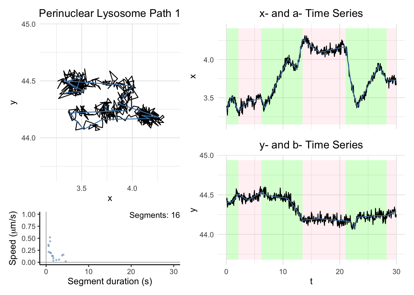
| Version | Author | Date |
|---|---|---|
| 380b9e2 | Ldo3 | 2025-10-15 |
The black line denotes the trajectory in the x-y coordinate plane and the time series for each coordinate. The blue line in each figure represents the inferred anchor position. Each green panel denotes a Motile segment, and each pink panel denotes a Stationary segment. Here, we used a threshold of \(0.1\mu\)m/s to label a segment as stationary/motile.
CPLASS_paths
# We will run on the 21PF data set with 3 paths.
subdata = data%>%filter(index_path%in%c(1,2,3)) #contains 3 paths
cplass_path = list()
for (i in 1:3)
{
     path = subdata %>% filter(index_path == i)
     t = path$t
     x = path$x
     y = path$y
     time_rate = min(diff(t))
     cplass_path[[i]] = CPLASS(t,x,y,iter_max = 2000)
}
saveRDS(cplass_path,file="output/Example_3_paths_Periphery.rds")
Visualization
Since we have a lot of paths here, it is better to save the plots into a pdf file to see them all together. The follow code will help us to do so. The output looks like this Real21PF_gallery.
path_list = cplass_path


file_list = c("21PF")
filestub = paste0("output/Real",file_list[1])
outfile = paste0(filestub,"_gallery.pdf")


motor = "Perinuclear Lysosomes" #change the name to the name of your data

pdf_output = TRUE

if (pdf_output == TRUE){
  pdf(outfile,onefile = TRUE,width=7,height=5)
}

dist_max = c()
t_max = c()
speed_max = c()

for (i in 1:length(path_list)){
  path = path_list[[i]]$path_inferred
  segments = path_list[[i]]$segments_inferred
  speed_max = c(speed_max,max(path_list[[i]]$segments_inferred$speeds))

  dist_max = c(dist_max,max(c(max(path$x)-min(path$x)),
                            max((path$y)-min(path$y))))
  t_max = c(t_max,max(path$t) - min(path$t))
}
xy_width = 1.2*max(dist_max)
t_lim = c(0,ceiling(max(t_max)))
max_speed = ceiling(max(speed_max))

for (i in 1:length(path_list)){
  if (i %% 20 == 0){
    print(paste("Working on path",i))
  }


  dashboard = plot_path_inferred(path_list[[i]],xy_width,t_lim, motor, max_speed)
  print(dashboard)


}

if (pdf_output == TRUE){
  dev.off()
}
sessionInfo()R version 4.5.1 (2025-06-13)
Platform: aarch64-apple-darwin20
Running under: macOS Ventura 13.1
Matrix products: default
BLAS: /Library/Frameworks/R.framework/Versions/4.5-arm64/Resources/lib/libRblas.0.dylib
LAPACK: /Library/Frameworks/R.framework/Versions/4.5-arm64/Resources/lib/libRlapack.dylib; LAPACK version 3.12.1
locale:
[1] en_US.UTF-8/en_US.UTF-8/en_US.UTF-8/C/en_US.UTF-8/en_US.UTF-8
time zone: America/Chicago
tzcode source: internal
attached base packages:
[1] parallel stats graphics grDevices utils datasets methods
[8] base
other attached packages:
[1] kableExtra_1.4.0 knitr_1.50 igraph_2.1.4 here_1.0.1
[5] ggthemes_5.1.0 earth_5.3.4 plotmo_3.6.4 plotrix_3.8-4
[9] Formula_1.2-5 glmnet_4.1-10 Matrix_1.7-3 doParallel_1.0.17
[13] iterators_1.0.14 foreach_1.5.2 patchwork_1.3.2 lubridate_1.9.4
[17] forcats_1.0.0 stringr_1.5.1 dplyr_1.1.4 purrr_1.1.0
[21] readr_2.1.5 tidyr_1.3.1 tibble_3.3.0 ggplot2_3.5.2
[25] tidyverse_2.0.0 limSolve_2.0.1 pracma_2.4.4 matrixcalc_1.0-6
[29] Rlab_4.0 workflowr_1.7.2
loaded via a namespace (and not attached):
[1] tidyselect_1.2.1 viridisLite_0.4.2 farver_2.1.2 fastmap_1.2.0
[5] promises_1.3.3 digest_0.6.37 timechange_0.3.0 lifecycle_1.0.4
[9] survival_3.8-3 processx_3.8.6 magrittr_2.0.3 compiler_4.5.1
[13] rlang_1.1.6 sass_0.4.10 tools_4.5.1 yaml_2.3.10
[17] labeling_0.4.3 bit_4.6.0 xml2_1.4.0 RColorBrewer_1.1-3
[21] withr_3.0.2 grid_4.5.1 git2r_0.36.2 scales_1.4.0
[25] MASS_7.3-65 cli_3.6.5 crayon_1.5.3 rmarkdown_2.29
[29] generics_0.1.4 rstudioapi_0.17.1 httr_1.4.7 tzdb_0.5.0
[33] cachem_1.1.0 splines_4.5.1 vctrs_0.6.5 jsonlite_2.0.0
[37] callr_3.7.6 hms_1.1.3 bit64_4.6.0-1 systemfonts_1.2.3
[41] jquerylib_0.1.4 glue_1.8.0 codetools_0.2-20 ps_1.9.1
[45] stringi_1.8.7 gtable_0.3.6 shape_1.4.6.1 later_1.4.3
[49] quadprog_1.5-8 pillar_1.11.0 htmltools_0.5.8.1 R6_2.6.1
[53] textshaping_1.0.1 rprojroot_2.1.1 vroom_1.6.5 lpSolve_5.6.23
[57] evaluate_1.0.4 lattice_0.22-7 httpuv_1.6.16 bslib_0.9.0
[61] Rcpp_1.1.0 svglite_2.2.1 whisker_0.4.1 xfun_0.53
[65] fs_1.6.6 getPass_0.2-4 pkgconfig_2.0.3