Visualization tools
Linh Do
Keisha J. Cook
Scott A. McKinley
Last updated: 2025-10-15
Checks: 7 0
Knit directory: CPLASS/
This reproducible R Markdown analysis was created with workflowr (version 1.7.2). The Checks tab describes the reproducibility checks that were applied when the results were created. The Past versions tab lists the development history.
Great! Since the R Markdown file has been committed to the Git repository, you know the exact version of the code that produced these results.
Great job! The global environment was empty. Objects defined in the global environment can affect the analysis in your R Markdown file in unknown ways. For reproduciblity it’s best to always run the code in an empty environment.
The command set.seed(20251014) was run prior to running
the code in the R Markdown file. Setting a seed ensures that any results
that rely on randomness, e.g. subsampling or permutations, are
reproducible.
Great job! Recording the operating system, R version, and package versions is critical for reproducibility.
Nice! There were no cached chunks for this analysis, so you can be confident that you successfully produced the results during this run.
Great job! Using relative paths to the files within your workflowr project makes it easier to run your code on other machines.
Great! You are using Git for version control. Tracking code development and connecting the code version to the results is critical for reproducibility.
The results in this page were generated with repository version a96e31a. See the Past versions tab to see a history of the changes made to the R Markdown and HTML files.
Note that you need to be careful to ensure that all relevant files for
the analysis have been committed to Git prior to generating the results
(you can use wflow_publish or
wflow_git_commit). workflowr only checks the R Markdown
file, but you know if there are other scripts or data files that it
depends on. Below is the status of the Git repository when the results
were generated:
Ignored files:
    Ignored:    .DS_Store
    Ignored:    data/.DS_Store
Note that any generated files, e.g. HTML, png, CSS, etc., are not included in this status report because it is ok for generated content to have uncommitted changes.
These are the previous versions of the repository in which changes were
made to the R Markdown (analysis/visualization_tools.Rmd)
and HTML (docs/visualization_tools.html) files. If you’ve
configured a remote Git repository (see ?wflow_git_remote),
click on the hyperlinks in the table below to view the files as they
were in that past version.
| File | Version | Author | Date | Message |
|---|---|---|---|---|
| html | a96e31a | Ldo3 | 2025-10-15 | update page |
| html | 380b9e2 | Ldo3 | 2025-10-15 | Build site. |
| Rmd | bebbb0b | Ldo3 | 2025-10-15 | wflow_publish(c("analysis/.")) |
In this pages, there are examples on how to plot paths and use Cumulative Speed Allocation (CSA) tool to compare between populations. For more details on CSA, we refer to the paper Cook, Rayens, Do, Payne and McKinley (2025).
We provide plot functions for visualizing trajectories (please click to the function for more details) including:
| Plot functions | Description |
|---|---|
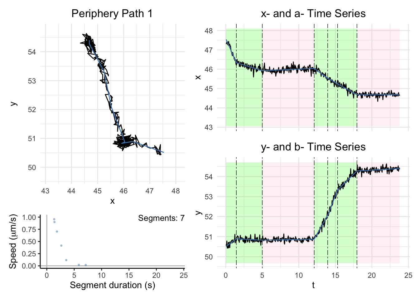
| plot_path_inferred() | Plot the segmented trajectories after running CPLASS |
| plot_path_actual_and_inferred() | Plot the actual overlap the inferred trajectories (for simulation data where we have the ground truth) |
| plot_csa() | Plot Cummulative Speed Allocations |
In this instructions, we continue using the
lysosome transport in the Periphery region of cells from
Payne’s lab. Please find the details on data collection here Rayens, Cook, McKinley,
and Payne.
paths = readRDS("data/21PF/CPLASS_21PF_250_paths_sSIC_with_speed_pen.rds") #load your data here

source("code/plot_functions.R")
source("code/csa_functions.R")
library("tidyverse")
library("ggplot2")
library("patchwork")
plot_path_inferred
Plot a single path
path_index = c(49)
# # If you want to select a certain path, use these lines
path_list = list(paths[[path_index]])

dist_max = c()
t_max = c()
speed_max = c()
motor ="Periphery" #change the name for your data

for (i in 1:length(path_list)){
  path = path_list[[i]]$path_inferred
  segments = path_list[[i]]$segments_inferred
  speed_max = c(speed_max,max(path_list[[i]]$segments_inferred$speeds))

  dist_max = c(dist_max,max(c(max(path$x)-min(path$x)),
                            max((path$y)-min(path$y))))
  t_max = c(t_max,max(path$t) - min(path$t))
}
xy_width = 1.2*max(dist_max)
t_lim = c(0,ceiling(max(t_max)))
max_speed = ceiling(max(speed_max))

for (i in 1:length(path_list)){
  if (i %% 20 == 0){
    print(paste("Working on path",i))
  }

  dashboard = plot_path_inferred(path_list[[i]],xy_width,t_lim, motor, max_speed, title_ind = path_index, show_time_changes = TRUE)

  print(dashboard)

}
| Version | Author | Date |
|---|---|---|
| 380b9e2 | Ldo3 | 2025-10-15 |
Plot all paths and create a gallery
The following code will help to save all of paths into a .pdf gallery. The output looks like this Periphery_gallery.
pdf_output = TRUE
path_list = paths

dist_max = c()
t_max = c()
speed_max = c()
motor ="Periphery"

if (pdf_output == TRUE){

  outfile = paste0("output/",motor,"_gallery.pdf")

  pdf(outfile,onefile = TRUE,width=7,height=5)
}


for (i in 1:length(path_list)){
  path = path_list[[i]]$path_inferred
  segments = path_list[[i]]$segments_inferred
  speed_max = c(speed_max,max(path_list[[i]]$segments_inferred$speeds))

  dist_max = c(dist_max,max(c(max(path$x)-min(path$x)),
                            max((path$y)-min(path$y))))
  t_max = c(t_max,max(path$t) - min(path$t))
}
xy_width = 1.2*max(dist_max)
t_lim = c(0,ceiling(max(t_max)))
max_speed = ceiling(max(speed_max))

for (i in 1:length(path_list)){
  if (i %% 20 == 0){
    print(paste("Working on path",i))
  }

  dashboard = plot_path_inferred(path_list[[i]],xy_width,t_lim, motor, max_speed)

  print(dashboard)

}
if (pdf_output == TRUE){
  dev.off()
}
plot_path_actual_and_inferred
This function is useful for evaluation the performance of CPLASS inferred trajectories on the simulation data sets.
Plot a single path
paths = readRDS("data/sim13CKP/Sim13_CKP_25Hz_cplass_with_speed_theory.rds")
path_index = c(15)
# # If you want to select a certain path, use these lines
path_list = list(paths[[path_index]])

dist_max = c()
t_max = c()
speed_max = c()
motor ="Simulation: Base" #change the name for your data

for (i in 1:length(path_list)){
  path = path_list[[i]]$path_inferred
  segments = path_list[[i]]$segments_inferred
  speed_max = c(speed_max,max(path_list[[i]]$segments_inferred$speeds))

  dist_max = c(dist_max,max(c(max(path$x)-min(path$x)),
                            max((path$y)-min(path$y))))
  t_max = c(t_max,max(path$t) - min(path$t))
}
xy_width = 1.2*max(dist_max)
t_lim = c(0,ceiling(max(t_max)))
max_speed = ceiling(max(speed_max))

for (i in 1:length(path_list)){
  if (i %% 20 == 0){
    print(paste("Working on path",i))
  }

  dashboard = plot_path_actual_and_inferred(path_list[[i]],xy_width,t_lim)

  print(dashboard)

}
Warning: Removed 2 rows containing missing values or values outside the scale range
(`geom_path()`).
Removed 2 rows containing missing values or values outside the scale range
(`geom_path()`).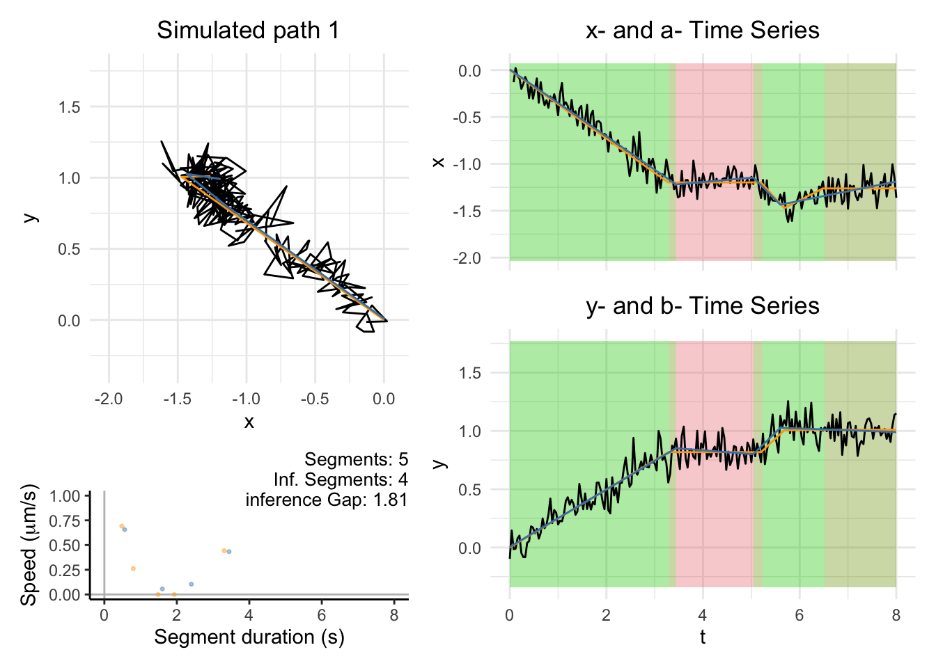
| Version | Author | Date |
|---|---|---|
| 380b9e2 | Ldo3 | 2025-10-15 |
Plot all paths and create a gallery
The following code will help to save all of paths into a .pdf gallery. The output looks like this Simulated_base_gallery.
pdf_output = TRUE
path_list = paths

dist_max = c()
t_max = c()
speed_max = c()
motor ="CKP13"

if (pdf_output == TRUE){

  outfile = paste0("docs/output/",motor,"_gallery.pdf")

  pdf(outfile,onefile = TRUE,width=7,height=5)
}


for (i in 1:length(path_list)){
  path = path_list[[i]]$path_inferred
  segments = path_list[[i]]$segments_inferred
  speed_max = c(speed_max,max(path_list[[i]]$segments_inferred$speeds))

  dist_max = c(dist_max,max(c(max(path$x)-min(path$x)),
                            max((path$y)-min(path$y))))
  t_max = c(t_max,max(path$t) - min(path$t))
}
xy_width = 1.2*max(dist_max)
t_lim = c(0,ceiling(max(t_max)))
max_speed = ceiling(max(speed_max))

for (i in 1:length(path_list)){
  if (i %% 20 == 0){
    print(paste("Working on path",i))
  }

  dashboard = plot_path_actual_and_inferred(path_list[[i]],xy_width,t_lim)

  print(dashboard)

}
if (pdf_output == TRUE){
  dev.off()
}
plot_csa
The following is the code to reproduce the Figure 8 in CPLASS paper (will be available soon) where we create CSA plots one for comparing lysosomal transport in perinuclear and periphery regions and one for comparing the sucrose-treated groups restricted to the periphery rgion of the cell. Please see Rayens, Cook, McKinley, and Payne for more details on the data, and Cook, Rayens, Do, Payne , McKinley for the calculation of CSA.
pdf_output = TRUE
folder_name = c("data/21PF/", "data/20PFS_and_PFL/")
real_data_file1 = paste0(folder_name[1],"CPLASS_21PN_250_paths_sSIC_with_speed_pen.rds")
real_data_file2 = paste0(folder_name[1],"CPLASS_21PF_250_paths_sSIC_with_speed_pen.rds")

real_path_list1 = readRDS(real_data_file1)
real_path_list2 = readRDS(real_data_file2)


cohort_list = c("Control Perinuclear",
                "Control Periphery")
color_list = c("Control Perinuclear" = "#1B9E77",
               "Control Periphery" ="#377EB8")

pdf_output = TRUE

##### Create Segment Summary ####
segment_summary = summarize_segments_inferred(real_path_list1,cohort_list[1])
segment_summary = bind_rows(segment_summary,
summarize_segments_inferred(real_path_list2,cohort_list[2]))

max_speed = min(1.2,max(segment_summary$speeds))

# Assumes theta is the same for all frame rates involved
speed_mesh = seq(0,max_speed,length = 200)
ds = speed_mesh[2] - speed_mesh[1]
subsample_size = 200
num_subsamples = 30

csa1 = tibble()

#### Bootstrap CSA for Real Data 1 ####
for (m in 1:num_subsamples){
    subsample = sample(1:length(real_path_list1),subsample_size,replace = TRUE)
    path_subsample = list()
    for (i in 1:length(subsample)){
      path_subsample[[i]] = real_path_list1[[subsample[i]]]
    }
    this_segments_summary = summarize_segments_inferred(path_subsample,"Sample")
    this_csa = compute_csa(this_segments_summary, speed_mesh)$csa
    csa1 = bind_rows(csa1,
                tibble(
                  s = speed_mesh,
                  csa = this_csa,
                  dcsa = c(diff(this_csa)/ds,0),
                  error = NA,
                  error_pct = NA,
                  label = cohort_list[1],
                  Hz = 20,
                  subsample = m
                ))
}


csa2 = tibble()
#### Bootstrap CSA for Real Data 2 ####
for (m in 1:num_subsamples){
    subsample = sample(1:length(real_path_list2),subsample_size,replace = TRUE)
    path_subsample = list()
    for (i in 1:length(subsample)){
      path_subsample[[i]] = real_path_list2[[subsample[i]]]
    }
    this_segments_summary = summarize_segments_inferred(path_subsample,"Sample")
    this_csa = compute_csa(this_segments_summary, speed_mesh)$csa
    csa2 = bind_rows(csa2,
                tibble(
                  s = speed_mesh,
                  csa = this_csa,
                  dcsa = c(diff(this_csa)/ds,0),
                  error = NA,
                  error_pct = NA,
                  label = cohort_list[2],
                  Hz = 20,
                  subsample = m
                ))
}


csa_both = bind_rows(csa1,csa2)

csa_both = csa_both %>% mutate(cohort = paste(label,subsample))

p_csa_compare1 = ggplot(csa_both %>% filter(label == cohort_list[1] |
                                      label == cohort_list[2]))+
  geom_line(aes(x = s, y = csa, col = label, group = cohort))+
  # ggtitle("Lysosome Periphery Large vs Small")+
  ylab("Cumulative Speed Allocation")+xlab(expression(paste("Speed (",mu,"m/sec)")))+
  scale_color_manual(values = color_list)+
  theme_minimal()+
     theme(
    legend.position = c(0.8, 0.2),  # Adjust position inside the plot
    legend.background = element_rect(fill = "white", color = "black")
  )+labs(color = NULL)
Warning: A numeric `legend.position` argument in `theme()` was deprecated in ggplot2
3.5.0.
ℹ Please use the `legend.position.inside` argument of `theme()` instead.
This warning is displayed once every 8 hours.
Call `lifecycle::last_lifecycle_warnings()` to see where this warning was
generated.print(p_csa_compare1)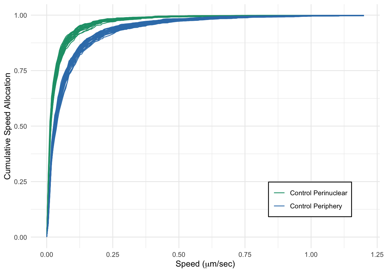
| Version | Author | Date |
|---|---|---|
| 380b9e2 | Ldo3 | 2025-10-15 |
pdf_output = TRUE
real_data_file1 = paste0(folder_name[2],"CPLASS_20PFL_250_paths_sSIC_with_speed_pen.rds")
real_data_file2 = paste0(folder_name[2],"CPLASS_20PFS_250_paths_sSIC_with_speed_pen.rds")

real_path_list1 = readRDS(real_data_file1)
real_path_list2 = readRDS(real_data_file2)

cohort_list = c("Sucrose Large",
                "Sucrose Small")
color_list = c("Sucrose Large" = "#1B9E77",
               "Sucrose Small" ="#377EB8")

pdf_output = TRUE


##### Create Segment Summary ####
segment_summary = summarize_segments_inferred(real_path_list1,cohort_list[1])
segment_summary = bind_rows(segment_summary,
                            summarize_segments_inferred(real_path_list2,cohort_list[2]))


max_speed = min(1.2,max(segment_summary$speeds))

# Assumes theta is the same for all frame rates involved
speed_mesh = seq(0,max_speed,length = 200)
ds = speed_mesh[2] - speed_mesh[1]
subsample_size = 200
num_subsamples = 30

csa1 = tibble()
#### Bootstrap CSA for Real Data 1 ####
for (m in 1:num_subsamples){
    subsample = sample(1:length(real_path_list1),subsample_size,replace = TRUE)
    path_subsample = list()
    for (i in 1:length(subsample)){
      path_subsample[[i]] = real_path_list1[[subsample[i]]]
    }
    this_segments_summary = summarize_segments_inferred(path_subsample,"Sample")
    this_csa = compute_csa(this_segments_summary, speed_mesh)$csa
    csa1 = bind_rows(csa1,
                tibble(
                  s = speed_mesh,
                  csa = this_csa,
                  dcsa = c(diff(this_csa)/ds,0),
                  error = NA,
                  error_pct = NA,
                  label = cohort_list[1],
                  Hz = 20,
                  subsample = m
                ))
}


csa2 = tibble()
#### Bootstrap CSA for Real Data 2 ####
for (m in 1:num_subsamples){
    subsample = sample(1:length(real_path_list2),subsample_size,replace = TRUE)
    path_subsample = list()
    for (i in 1:length(subsample)){
      path_subsample[[i]] = real_path_list2[[subsample[i]]]
    }
    this_segments_summary = summarize_segments_inferred(path_subsample,"Sample")
    this_csa = compute_csa(this_segments_summary, speed_mesh)$csa
    csa2 = bind_rows(csa2,
                tibble(
                  s = speed_mesh,
                  csa = this_csa,
                  dcsa = c(diff(this_csa)/ds,0),
                  error = NA,
                  error_pct = NA,
                  label = cohort_list[2],
                  Hz = 20,
                  subsample = m
                ))
}


csa_both = bind_rows(csa1,csa2)
csa_both = csa_both %>% mutate(cohort = paste(label,subsample))

p_csa_compare2 = ggplot(csa_both %>% filter(label == cohort_list[1] |
                                      label == cohort_list[2]))+
  geom_line(aes(x = s, y = csa, col = label, group = cohort))+
  # ggtitle("Lysosome Periphery Large vs Small")+
  ylab("Cumulative Speed Allocation")+xlab(expression(paste("Speed (",mu,"m/sec)")))+
  scale_color_manual(values = color_list)+
  theme_minimal()+
     theme(
    legend.position = c(0.85, 0.2),  # Adjust position inside the plot
    legend.background = element_rect(fill = "white", color = "black")
  )+labs(color = NULL)
print(p_csa_compare2)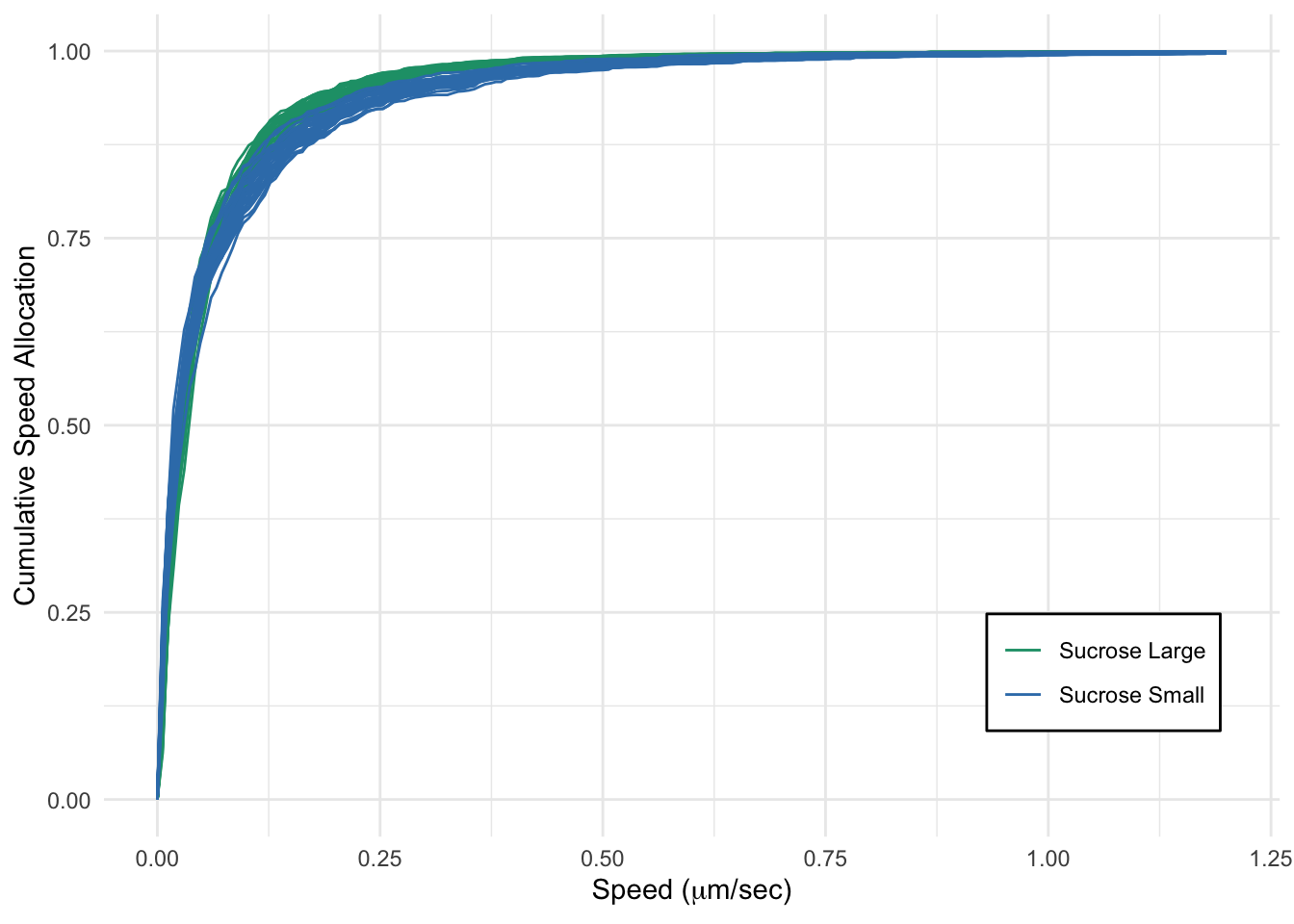
| Version | Author | Date |
|---|---|---|
| 380b9e2 | Ldo3 | 2025-10-15 |
p_csa_full = (p_csa_compare1 + p_csa_compare2)

if (pdf_output == TRUE){
  outfile = paste0("docs/output/Figure_CSA_compare_PN_PF_PFL_PFS.pdf")
  pdf(outfile,onefile = TRUE,width=9.5,height=3)
}

print(p_csa_full)

if (pdf_output == TRUE){
  dev.off()
}
quartz_off_screen
2
sessionInfo()R version 4.5.1 (2025-06-13)
Platform: aarch64-apple-darwin20
Running under: macOS Ventura 13.1
Matrix products: default
BLAS: /Library/Frameworks/R.framework/Versions/4.5-arm64/Resources/lib/libRblas.0.dylib
LAPACK: /Library/Frameworks/R.framework/Versions/4.5-arm64/Resources/lib/libRlapack.dylib; LAPACK version 3.12.1
locale:
[1] en_US.UTF-8/en_US.UTF-8/en_US.UTF-8/C/en_US.UTF-8/en_US.UTF-8
time zone: America/Chicago
tzcode source: internal
attached base packages:
[1] stats graphics grDevices utils datasets methods base
other attached packages:
[1] patchwork_1.3.2 lubridate_1.9.4 forcats_1.0.0 stringr_1.5.1
[5] dplyr_1.1.4 purrr_1.1.0 readr_2.1.5 tidyr_1.3.1
[9] tibble_3.3.0 ggplot2_3.5.2 tidyverse_2.0.0 workflowr_1.7.2
loaded via a namespace (and not attached):
[1] sass_0.4.10 generics_0.1.4 stringi_1.8.7 hms_1.1.3
[5] digest_0.6.37 magrittr_2.0.3 timechange_0.3.0 evaluate_1.0.4
[9] grid_4.5.1 RColorBrewer_1.1-3 fastmap_1.2.0 rprojroot_2.1.1
[13] jsonlite_2.0.0 processx_3.8.6 whisker_0.4.1 ps_1.9.1
[17] promises_1.3.3 httr_1.4.7 scales_1.4.0 jquerylib_0.1.4
[21] cli_3.6.5 crayon_1.5.3 rlang_1.1.6 withr_3.0.2
[25] cachem_1.1.0 yaml_2.3.10 tools_4.5.1 tzdb_0.5.0
[29] httpuv_1.6.16 vctrs_0.6.5 R6_2.6.1 lifecycle_1.0.4
[33] git2r_0.36.2 fs_1.6.6 pkgconfig_2.0.3 callr_3.7.6
[37] pillar_1.11.0 bslib_0.9.0 later_1.4.3 gtable_0.3.6
[41] glue_1.8.0 Rcpp_1.1.0 xfun_0.53 tidyselect_1.2.1
[45] rstudioapi_0.17.1 knitr_1.50 farver_2.1.2 htmltools_0.5.8.1
[49] labeling_0.4.3 rmarkdown_2.29 compiler_4.5.1 getPass_0.2-4